Condensed Matter Physics

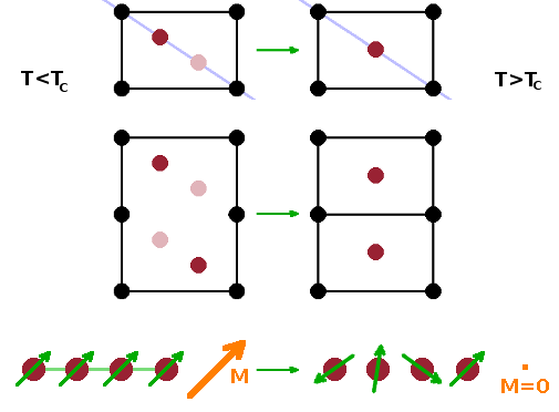
The fundamental idea of Landau theory is to define an order parameter, Q (or sometimes ζ), i.e. a measurable property that traces a system's approach to a phase transition. Many different physical properties can be used as an order parameter for different kinds of transition, and usually there are different properties which could equally well be used for a given transition. The point is that it is something that varies sharply at the transition point and can be measured easily. Examples include:

density

As we have seen, the increase in symmetry in the high-temperature phase during crystallographic transitions leads to a reduction in density. Therefore density can be used as an order parameter for such transitions.

site occupancies

Site occupancies can be measured indirectly, for example by phonon spectroscopy. If a site becomes vacant or is only occupied part of the time on the high-temperature side of a displacive transition, the occupancy fraction can be used as an order parameter.

Bragg peak intensities

Diffraction peaks disappear as a consequence of systematic absences in the case of centred unit cells. Therefore, Bragg peaks will vanish during a displacive phase transition if the high-temperature phase has a centred lattice (as in the example discussed).

Bragg peak positions

If inter-atomic distances change during a phase transition, Bragg peaks will move as a result.

magnetisation, polarisation

In transitions between ferromagnetic and paramagnetic states (or their electrical analogues), the magnetisation (polarisation) will vanish abruptly because the individual magnetic moment (dipole moment) vectors cancel out in the disordered phase, making a good order parameter.

resistivity

Resistivity is a useful order parameter in transitions involving superconductors since it vanishes below the transition point.

...

In order for all these different observable properties to be used as order parameters, they need to be scaled to be within $[0\cdots 1]$, where $Q=0$ corresponds to the disordered phase. Below the transition, in the ordered phase, the order parameter rises to its low-temperature limit of 1. For example, in the case of the displacive transition shown, the distance of the atom from the centre position along the diagonal (as measured by Bragg angle) is 0 in the high-temperature phase and gradually increases upon cooling below $T_c$ as the atom settles in its asymmetric potential well.

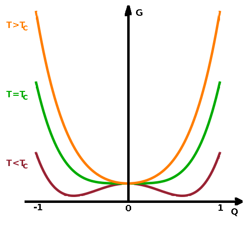
The order parameter is normalised in such a way that $Q=0$ above the transition and $Q=1$ in the limit of $T\to\mathrm{0\,K}$. The free enthalpy of the thermodynamically stable phase has a minimum at the value of the order parameter for the given temperature (or whichever state variable is being changed). As a result, we have

• $T\gt T_c$: one minimum at $Q=0$
• $T\lt T_c$: two minima at $|Q|\gt 0$

For a symmetric problem such as the displacement of an atom along the cell diagonal, Taylor expansion of the free enthalpy produces $$G(Q)=G_0+\frac{1}{2}aQ^2+\frac{1}{4}bQ^4+\cdots$$ In a second-order phase transition, the coefficient of the second-order expansion term $a$ varies smoothly with temperature and hinges on $T_c$: $$a(T)=a_0(T-T_c)\qquad,$$ i.e. the strength of the term depends on how far away from the transition temperature $T_c$ the system is. By inserting this into the expanded $G(Q)$ expression, we have: $$G(Q)=G_0+\frac{1}{2}a_0(T-T_c)Q^2+\frac{1}{4}bQ^4+\cdots$$ We find the minima and maxima of $G(Q)$ by finding the points where its derivative is zero: $$\frac{\partial G}{\partial Q}=a_0(T-T_c)Q+bQ^3\overset{!}{=}0$$ This produces the solutions:

$$Q=0\textrm{ - minimum for }T\gt T_c\textrm{, maximum for }T\lt T_c\textrm{, and}$$ $$Q=\pm\sqrt{\frac{a_0}{b}(T_c-T)}\textrm{ - unphysical (since imaginary) for }T\gt T_c\textrm{, minima for }T\lt T_c\textrm{.}$$

Therefore, we can see that the two free energy minima gradually move towards $Q=0$ as the system heats up towards $T_c$. From $T_c$ onwards, the free energy minimum remains fixed at $Q=0$, indicative of the high-temperature, high-symmetry phase.

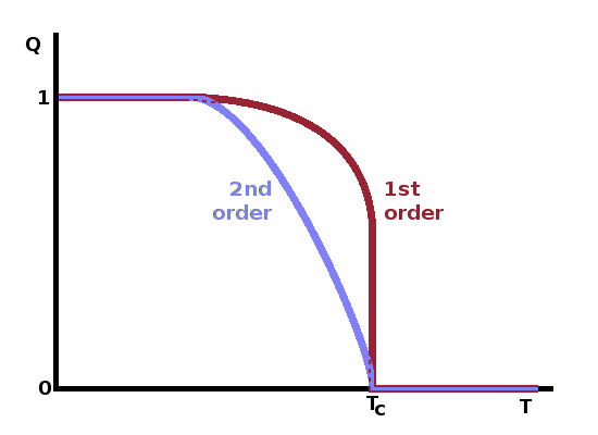
Clearly this approach produces the required temperature dependence of the order parameter: At the lowest temperatures, $Q$ approaches one, falling gradually towards zero at $T_c$. The rate of change increases as the phase transition is approached. Above the transition point, the order parameter remains fixed at zero.

In a first-order phase transition, the order parameter drops to zero instantly at the transition point after gradually decreasing somewhat from the low-temperature limit of one. The difficulty in determining the order of a phase transition experimentally is mirrored here: with finite precision of the temperature measurement, it is impossible to tell whether the angle between the $G(Q)$ function and the temperature axis is 90^o (1st order) or marginally larger (2nd order).

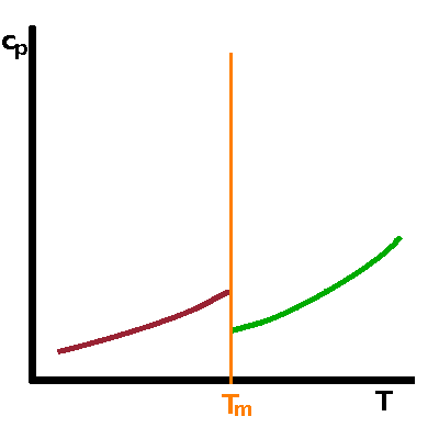
The heat capacity can be calculated from the entropy by evaluating $$c_p=T\frac{\partial S}{\partial T}\qquad.$$ By using the transition entropy, $\Delta S$, in this formula we can work out the additional contribution to the heat capacity that results from the phase transition. This is in addition to the heat capacity of the material itself. Therefore, the transition-related component of the heat capacity is obtained by evaluating the slope of the entropy at the transition: $$c_p^{\mathrm{phtr}}=T\frac{\partial(\Delta S)}{\partial T}=-T\frac{1}{2}a_0\frac{\partial Q^2}{\partial T}\qquad.$$ Here we can use the roots of $Q(T)$ we've found above by differentiating the free enthalpy. Below $T_c$, we have found $$Q(T)=\pm\sqrt{\frac{a_0}{b}(T_c-T)}\qquad\textrm{, so}$$ $$c_p^{\mathrm{phtr}}=-\frac{1}{2}a_0T\frac{\partial}{\partial T}\left(\frac{a_0}{b}(T_c-T)\right)=\frac{a_0^2T}{2b}\qquad.$$ Since $Q(T)=0$ if $T\gt T_c$, the transition-related contribution to $c_p$ above the transition point is zero, i.e. $$\Delta c_p=c_p^{\mathrm{phtr}}$$ determines the size of the step in the heat capacity at the second-order phase transition.

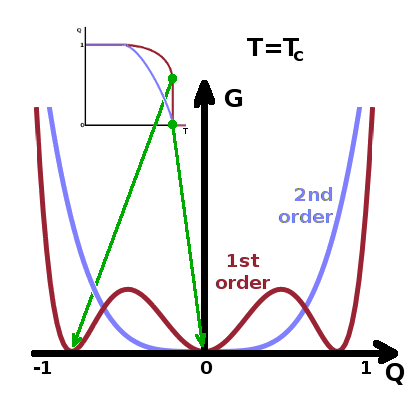
When considering the temperature dependence of the order parameter, $Q(T)$, it is clear that the function is single-valued only for second-order transitions. For first-order transitions, the order parameter drops vertically at the transition temperature. Therefore, the free enthalpy must have at least one additional minimum within the range $[0\dots 1]$ of the order parameter. This cannot be achieved if the Taylor expansion of $G(Q)$ is truncated after the quartic ($Q^4$) term. We therefore include the $Q^6$ term as well: $$G(Q)=\frac{1}{2}a_0(T-T_c)Q^2-\frac{1}{4}bQ^4+\frac{1}{6}cQ^6\qquad .$$ The signs of the expanasion terms alternate, producing the required pattern.
Different sources define the coefficients slightly differently, so the following formulae may look a little different depending on how $a,b,c$ are introduced.

To find the values of the order parameter at which the free enthalpy is minimal, we need to find the zeroes of the derivative of $G(Q)$ with respect of $Q$: $$\frac{\partial G}{\partial Q}=a_0(T-T_c)Q-bQ^3+cQ^5\stackrel{!}{=}0\qquad .$$

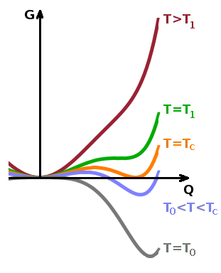
The solutions are: $$Q=0\qquad\textrm{or}$$ $$a_0(T-T_c)-bQ^2+cQ^4=0\qquad .$$ The latter can be solved as a quadratic equation in terms of $Q^2$ as the variable: $$(Q^2)^2-\frac{b}{c}Q^2+\frac{a_0}{c}(T-T_c)=0\qquad,$$ leading to the solutions $$Q^2=\frac{b}{2c}\pm\sqrt{\frac{b^2}{4c^2}-\frac{a_0}{c}(T-T_c)}\quad.$$ This can be simplified somewhat by including the $2c$ in the root: $$Q^2=\frac{1}{2c}\left(b\pm\sqrt{b^2-4a_0c(T-T_c)}\right)\qquad.$$

Since the free energy is a real function, the inner root must be real, so $$b^2\ge 4a_0c(T-T_c)\qquad.$$ Solving this for the temperature yields: $$T\le T_1=T_c+\frac{b^2}{4a_0c}\qquad,$$ where the spinodal temperature, $T_1$, is the upper limit of the temperature range in which the low-temperature phase can co-exist as a metastable form alongside the thermodynamically stable high-temperature phase. In terms of $G(Q)$, this is the point at which a second minimum at $Q\gt 0$ forms. This is a local minimum, i.e. the free enthalpy of the high-temperature phase ($Q=0$) is lower still. At the transition temperature, $T_c$, the free enthalpy is $G=0$ for both minima, i.e. both phases are in thermodynamic equilibrium. Below the transition temperature, the low-temperature phase becomes stable while the high-temperature phase can co-exist metastably - its local minimum at $Q=0$ has a larger value than that of the stable phase. At the binodal temperature, $T_0$, the sign the local minimum of the high-temperature phase flips over and becomes a local maximum. Below $T_0$, the high-temperature phase cannot exist even as a metastable phase.

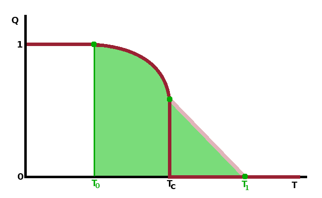
Unless terms beyond $Q^6$ are included in the analysis, the two metastable regions are symmetrical - $T_0$ is as far below $T_c$ as $T_1$ is above it. The metastable regimes come about because of structural fluctuations which reach their maximum extent at $T_c$.

The schematic diagram shows the variation of the order parameter with temperature near a first-order phase transition, including the two coexistence regions and the gradual approach to zero of the order parameter of the metastable low-temperature phase as the sample is heated towards the spinodal temperature.