
If a paramagnetic material is placed inside a magnetic field, the magnetic moments of atoms tend to align with the external field. However, as soon as the external field is removed, thermal disorder will disrupt the alignment very quickly. In a ferromagnet, on the other hand, the alignment persists after the field is removed. This is caused by an interaction between the individual moments rather than just between the individual moments and the external field.
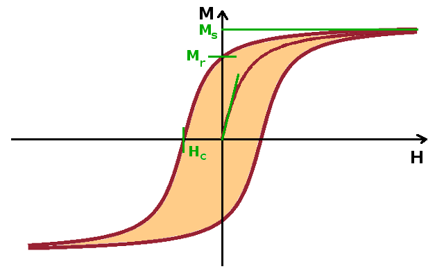
When a ferromagnetic material is placed in an external field for the first time (purple curve starting at the origin), the magnetisation begins to build up linearly at first (green tangent shown). After a while, a further increasing field begins to have diminishing effects on the resulting magnetisation, so the curve begins to level off and ultimately reaches saturation, $M_s$, no matter whether the field is held constant or increased any further.
When the external field is reduced again, the magnetisation is maintained at first, and then gradually decreases as the field subsides. When the external field reaches zero, the magnetisation is still positive. The level of magnetisation after switching off an external field is known as remanence, $M_r$. As the field is ramped up in the opposite direction, the magnetisation (now opposing the external field - top left quadrant) continues to diminish until it reaches zero. The external field needed to remove the magnetisation from a previously magnetised ferromagnet is the coercive field, $H_c$. As the field's magnitude continues to rise beyond this point, magnetisation parallel to the field builds up until saturation is reached again.
Once magnetised, the magnetisation continues to loop around the origin when the polarity of the field is cycled without ever returning to it. This infinite loop is known as hysteresis. The only way to return the material to a demagnetised state is to supply thermal or mechanical energy to the specimen.
The area enclosed by the hysteresis loop (shaded area in the Figure) is a measure of the amount of energy stored in the magnetic interaction. Hard magnets are materials with a high remanence and coercive field, thus a steeply sloping hysteresis curve enclosing a large area. These are good for magnetic storage devices, where two well-defined states need to be distinguished and protected against incidental change of state. The opposite, soft magnets are better suited to mechanical control applications (e.g. positioning) since they give finer control of the magnetisation via the applied field.
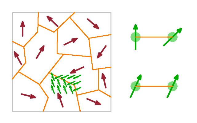
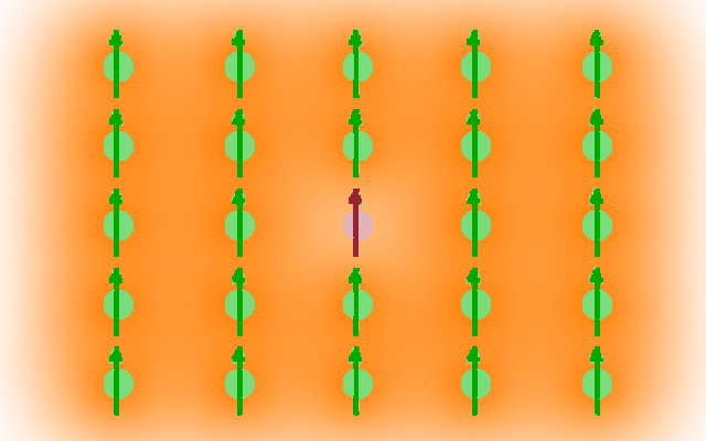
In a ferromagnetic material, the interaction between neighbouring moments is strong enough to overcome thermal fluctuations. Effectively, each moment aligns itself according to the magnetic field constituted by its neighbours. In a spontaneously magnetised material (i.e. in the absence of an external field) this alignment process occurs simultaneously in different parts of the sample, resulting in magnetic domains with uniform orientation of magnetic moments. Although structural grain boundaries can impair the dynamics of these domains, the size of the domains is largely independent of the crystalline grain structure: domains can transcend grain boundaries, and grains can contain multiple domains.
Domains are separated by Bloch walls. Again, these walls have no structural basis; they are simply the boundaries either side of which individual moments have a different orientation as they belong to adjacent domains. The moments near the Bloch walls have an increased amount of potential (magnetic) energy due to the fact that they have neighbours producing an opposing field, whichever way they orientate. This is known as magnetic frustration.
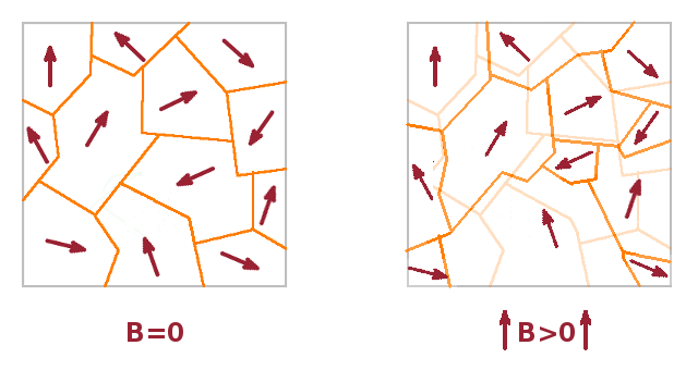
When a spontaneously magnetised ferromagnet is placed in an external magnetic field, the balance of interactions on the magnetic moments near the Bloch walls is disturbed. If the domain on one side of a Bloch wall is roughly aligned with the external field but the other domain isn't, the magnetic moments at the Bloch wall will be able to reduce their potential energy by reorientating to match the orientation of the favourable domain. Thus the favourable domains grow and the unfavourable ones shrink. Note that there is no wholesale re-orientation of domains, a process which would have a much higher activation energy than this piecemeal process. At saturation, all individual moments have flipped and the whole magnet consists of a single domain of moments aligned with the external field. If the field is subsequently switched off, domains will recur, but the orientation of the previous external field will remain the dominant component. This explains the remanence of the magnetised ferromagnet.
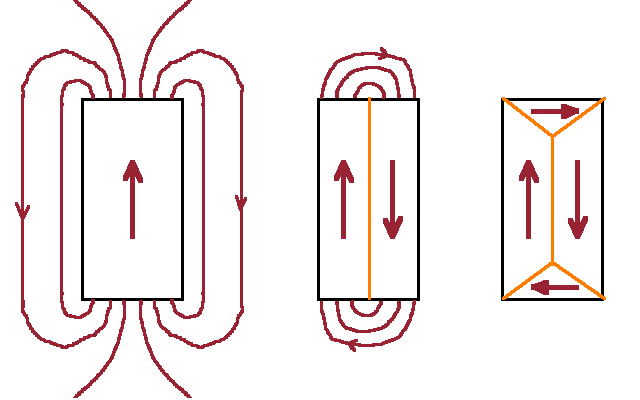
If a saturated ferromagnet consists of just one single domain, magnetic moments have to reorientate spontaneously to form new domains when the external field is removed. This process is driven by the reduction of the spread of the magnetic field supported by the magnetic structure of the ferromagnet. In its single-domain saturated state, the magnetic field spreads out far into the surrounding space, thereby interacting with magnetic moments and inducing currents elsewhere. The spread of the field and its interactions are reduced by growing an opposing domain such that field lines only connect adjacent domains at the ends of the magnet. A further reduction of the supported field can be achieved by terminal domains which keep the magnetic field confined to the magnet itself.
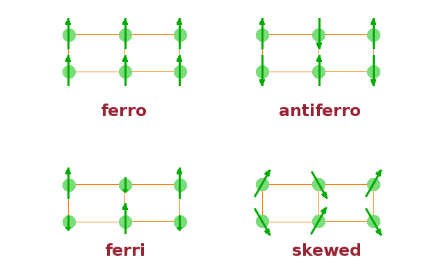
While the ferromagnetic state is the most important collective magnetic phenomenon, there are other interaction patterns that result in collective magnetism: In an antiferromagnet, adjacent moments orientate themselves in opposite direction, thus cancelling each other out - no net external magnetisation is observed. If there are two different chemical elements present in the sample, their total angular momentum and therefore magnetic moment will usually be different, resulting in moments of different magnitude on alternate lattice positions. This results in ferrimagnetism, where two distinct sub-lattices overlap. There are also other more complex forms of collective magnetism such as the skewed arrangement shown; all of these have in common an ordered periodic pattern of magnetic moments within each domain.
The magnetic ordering competes with thermal disorder. In energy terms, this means that the ordering prevails as long as the magnetic energy, $p_mB_{ex}$ is larger than the thermal energy, $k_BT$. This marks the phase transition between the ferromagnetic (ordered, low-temperature) phase and the paramagnetic (disordered, high-temperature) phase. The transition occurs at the Curie temperature, where magnetic and thermal energy are exactly balanced.
However, $B_{ex}$ isn't any external magnetic field here (as that would mean the transition would vanish in the absence of an external field), but rather an internal magnetic field in the material that characterises the interaction between the individual moments. This is known as the exchange field, a very large but short-range field constituted by nearby moments which interacts with the central magnetic moment. Each individual moment is subject to such an exchange field originating from its neighbours. On its local length scale, the exchange field is much stronger than any external field would be, of the order of $\mathrm{10^3T}$ locally.
The exchange field causes the susceptibility of the paramagnetic (high-temperature) phase of a ferromagnet to deviate from the Curie law usually observed in paramagnetic materials. The magnetisation of a ferromagnet above the transition temperature can be expressed in terms of the susceptibility $\chi_C$ of a paramagnet subject to the exchange field: $$M=\chi_C(B_0+B_{ex})\qquad,$$ where $B_0$ is the externally applied field. Using the Curie law, $\chi=\frac{C}{T}$ and the fact that the exchange field is due to the concerted effect of all the magnetic moments in the sample and therefore proportional to the magnetisation, $B_{ex}=\lambda M$, we have $$M=\frac{C(B_0+\lambda M)}{T}\qquad.$$
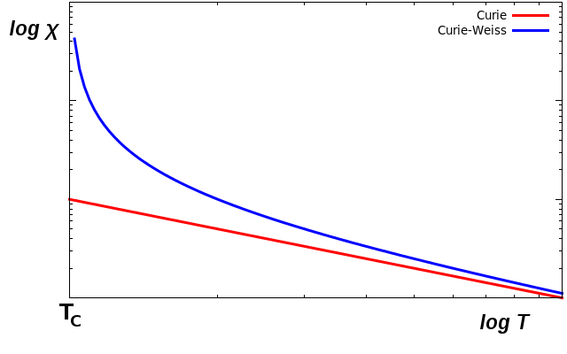
The susceptibility $\chi_{CW}$ of the paramagnetic phase of a ferromagnet is, as usual, defined relative to the external field only, and by re-arranging the above: $$MT=CB_0+\lambda CM\quad\Leftrightarrow\quad M(T-\lambda C)=CB_0\qquad,$$ we can evaluate it as $$\chi_{CW}=\frac{M}{B_0}=\frac{C}{T-\lambda C}\qquad.$$ Thus, the susceptibility of the paramagnetic (high-temperature) phase of a ferromagnetic material depends on the temperature, but it's not the simple inverse relationship we know from the Curie law of paramagnetism. Instead, the Curie-Weiss law applies: $$\chi_{CW}=\frac{C}{T-T_C}\qquad,$$ where $T_C$ is the Curie temperature, i.e. the critical temperature for the ferro-/paramagnetic transition, $C$ is the Curie constant of the paramagnetic phase, and $\lambda$ is the strength of the interaction between magnetic moments.
This means that the paramagnetic phase of a ferromagnetic material behaves in the same way as it approaches the Curie temperature from above as a paramagnetic material does when cooling towards zero Kelvin. One might say that a paramagnet is a ferromagnet whose Curie temperature is indistinguishable from absolute zero.
Given that the para-/ferro-magnetic transition is driven by the balance of magnetic (potential) and thermal (kinetic) energy and comes about due to the alignment of neighbouring magnetic moments, we can predict the probability $p_{\textrm{flip}}$ that a given moment will flip at any given time by considering the ratio of the two energies: $$p_{\textrm{flip}}=\exp\left(-\frac{W_{\textrm{mgn}}}{k_BT}\right)\qquad,$$ where $W_{\textrm{mgn}}$ can be any value within a range given by perfect parallel and anti-parallel alignment with the moment's neighbours. Any model of the domain structure of a ferromagnet based on this statistical approach is known as an Ising model, named after Ernst Ising, who first suggested this probabilistic procedure which lends itself to computer modelling. Alternatively, the magnetic energy can be calculated from the quantum-mechanical exchange integral of overlapping electron clouds of adjacent atoms, which again can be balanced with the thermal energy in the same way to produce alignment probabilities. This modelling approach is known as the Heisenberg model.
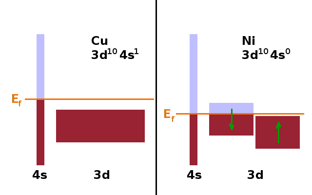
As in the case of paramagnetism in metals, conduction electrons and their band structure have implications for ferromagnetic materials, too. The Figure contrasts (a simplified schematic version of) the band structure of copper and nickel, two elements adjacent in the periodic table. Nickel has one electron less than copper; therefore the Fermi level (i.e. the highest occupied state in the limit of zero temperature) is a little lower in nickel.
As we know from the solution of the Schrödinger equation of the hydrogen atom, the energy of an electron is determined by the main quantum number, $n$. However, the interaction between the different electrons in atoms further down the periodic table results in shifts and splits of energy levels according to their orbital angular momentum quantum number, $l$ - indicated by letters like s,p,d,f... in the label of the respective state. How this comes about is covered in the section on the Central Field Approximation in the Atoms and Molecules lecture. As a result of these shifts, the 4s and the 3d states are at a comparable energy.
In copper, all the 3d states are occupied and the 4s band is half full at $T\to 0$. In nickel, there is one less electron, and as a result the Fermi level cuts through both the 4s and the 3d band, so the notional occupancy of 3d104s0 isn't quite correct. At this point, the magnetic exchange interaction becomes important: the 3d band splits into two sub-bands with opposing magnetic moment (and therefore magnetic quantum number, $m$). One orientation is energetically more favourable than the other, resulting in the parallel aligned sub-band being entirely below the Fermi level while the anti-parallel sub-band is only partially occupied. This produces as strong permanent magnetic moment from the excess magnetic moments.
Having considered the various forms of magnetism in materials, we can compare electric and magnetic properties and emphasise the many similarities.