
Braggs' law describes the constructive interference of parallel rays after reflection at a set of semi-transparent lattice planes. Each plane reflects a certain fraction of the incident wave and transmits the remainder. In an infinitely large crystal, the full beam will be reflected at one plane or another. However, if the crystal is only a few lattice planes thick, some of the beam will penetrate the whole crystal and will leave the grain before it is reflected. Therefore, fewer lattice planes contribute to the Bragg condition, and the peak is less well defined than for a perfect, infinitely large crystal, resulting in a broadened peak. Exactly how many lattice planes are needed before a particular finite crystal is indistinguishable from a perfect one depends on the wavelength of the radiation and the electron density (for x-ray diffraction) or scattering length density (for neutron diffraction) of the crystal.
ER van Hoek, R Winter
Amorphous silica and the intergranular structure of nano-crystalline silica
Phys Chem Glass 43C (2002) 80
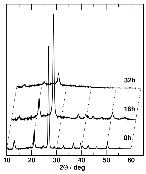
In order to see the effect of reduced particle size on the diffractograms, we can compare the x-ray diffraction patterns obtained from coarse-grained quartz sand with those of the same material after prolonged periods of high-energy ball milling. This technique involves filling a small amount of the sample in a vessel made from a very hard material (e.g. corundum, $\mathrm{Al_2O_3}$) together with a small ball made of the same material and shaking the vessel rapidly in three different spatial directions to cause a chaotic movement of the ball in the vessel. X-ray diffractograms are taken after varying periods of several hours to several days.
The most obvious effect on the diffractograms is the peak broadening, which can best be seen in the strongest peaks. Since peaks come in different sizes (magnitudes), it is important to determine peak widths in well-defined, comparable terms (generally, not just in diffraction). This is achieved by measuring the full width at half magnitude (fwhm) of the peak because the sides of the peak are steepest at half its height, minimising the error of the measurement. To do this, the level of the baseline of the peak is determined by connecting two points at the average level of the noise on either side of the peak. The magnitude of the peak is the vertical distance from the baseline (which may be slanted) to the maximum, so the fwhm of the peak is measured at the midpoint between the baseline and the maximum. This will produce values that can be compared even if the peaks involved in the comparison are very different in magnitude.
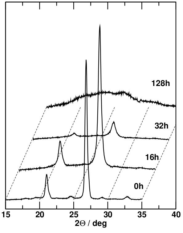
Peak broadening is noticeable after 16 hours of ball milling; after 32 hours, the extent of this broadening is such that the less intense Bragg peaks vanish in the noise. However, the stronger peaks are still clearly visible, and their fwhm can be determined. After 128 hours of ball milling, there are no obvious Bragg peaks left; instead there is a broad featureless background for which no fwhm can be determined.
The peak broadening of the individual Bragg peaks is due to the progressively more limited particle size and the smaller number of lattice planes contributing to the constructive interference that constitutes the Bragg condition. At the same time, the attrition of the material due to the milling process causes a higher proportion of the material to be in distorted grain boundary environments, which lack long-range periodicity. The 128-hour sample shows the end point of this process of amorphisation, i.e. complete loss of long-range order. However, even in an amorphous material, short-range order is maintained because the local environment (bond lengths and co-ordination polyhedra) are the same in crystalline and amorphous forms of the same composition. While there are no lattice planes and therefore no Bragg reflections, there are characteristic lengths such as bond lengths and typical sizes of groups of co-ordination polyhedra, whose mean values correspond to increased scattering amplitudes at certain angles, adding up to a broad amorphous peak.
Size broadening of diffraction peaks can be used to estimate the size of nanocrystals. To establish a relationship between particle size and fwhm of a Bragg peak, we start with Braggs' law. $$n\lambda=2d\sin{\theta}\qquad.$$ The column length, $L$, is the grain size in a particular crystallographic orientation. It must be an integer multiple of the lattice spacing in that direction: $$L=md\quad(m=2,3,4\dots)\qquad.$$ Thus Braggs' law becomes $$m\lambda=2L\sin{\theta}\qquad,$$ considering only first order ($n=1$) diffraction peaks. The total differential of a function is the sum of the partial derivatives of the function with respect to all its variables, each multiplied with the variation in that variable: $$\Delta f(x,y)=\frac{\partial f}{\partial x}\Delta x+\frac{\partial f}{\partial y}\Delta y\qquad.$$ With the wavelength fixed, there is nothing to differentiate on the left, but the right-hand side has two terms: $$0=\frac{\partial}{\partial L}\left(2L\sin\theta\right)\Delta L+\frac{\partial}{\partial\theta}\left(2L\sin\theta\right)\Delta\theta\\ =2\sin{\theta}\Delta L+2L\cos{\theta}\Delta\theta\qquad.$$ This can be solved for the column length: $$L=-\frac{\sin{\theta}\Delta L}{\cos{\theta}\Delta\theta}\qquad.$$ However, the column length can only change by multiples of the lattice spacing: $$\left|\Delta L\right|=d,$$ so we can substitute: $$L=\frac{\sin{\theta}\,d}{\cos{\theta}\Delta\theta}\qquad.$$ Finally, resubstitute Braggs' law to obtain $$L=\frac{\lambda}{2\cos{\theta}\Delta\theta}\qquad.$$ Diffractograms are recorded on a $2\theta$ scale owing to the fact that both incident and reflected ray make an angle of $\theta$ with the reflecting lattice plane. Therefore, the full width at half magnitude of a diffraction peak is $$\beta=\Delta(2\theta)=2\Delta\theta\qquad.$$ Substituting that produces the
$$\textbf{Scherrer equation}:\qquad L=\frac{K\lambda}{\beta\cos{\theta}}$$
relating the peak width and the grain size, where the shape factor, $K$, makes an adjustment for the shape of the grains. For unimpeded crystal growth, it is possible to calculate the shape factor for different structure types because of the different growth rates in different crystallographic orientations. However, this is impossible if crystal growth occurs in confined geometries or, as in the case of nanocrystalline materials prepared by ball milling, if large grains are broken up into nano-sized chunks. The shape factor is always close to 1, and in cases where it cannot be determined, a value of $K=0.9$ is often assumed. While this does produce a systematic error on the estimated particle size, it is reasonable to assume that the error affects all samples in a set equally if only peaks from the same material under different conditions are compared.
However, there are a few other caveats to consider when using the Scherrer equation. First, it is important to remember that $L$ is the column length in a particular crystallographic orientation, not necessarily the radius of the particle. Therefore, comparisons of $L$ values taken from Bragg peaks with different Miller indices are problematic. Another severe limitation is that the Scherrer equation assumes that the only cause for peak broadening is the finite grain size. However, there are other peak broadening mechanisms, in particular microstrain. Another factor contributing to the width of diffraction peaks is instrumental broadening, i.e. the divergence of the beam due to the beam optics and air scattering between the source and the detector. However, this can easily be corrected for by taking a reference measurement of a coarse-grained sample of the same crystal structure under the same conditions. If the peak shape is Gaussian, the correction is made on the basis of the squares of the fwhm of the sample and the reference material: $$\beta=\sqrt{\beta_{\mathrm{sample}}^2-\beta_{\mathrm{reference}}^2}\qquad.$$
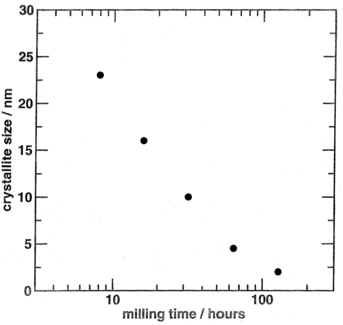
Returning to the ball-milled quartz case study, the column lengths calculated from the strongest Bragg reflection are shown in the Fig. as a function of milling time. The particle size decreases on a logarithmic time scale. By extrapolation of the first four data points, the particle size would be reduced to zero after about 100 hours, which is consistent with the observation that the sample milled for longer than that appears to have been amorphised altogether.
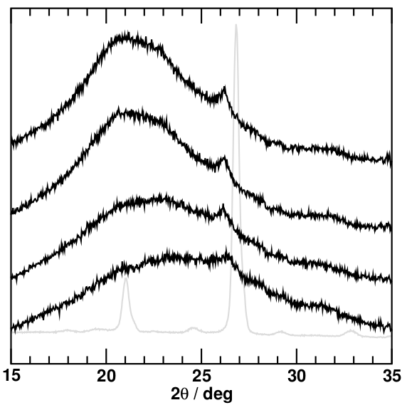
Once fully amorphised, the only way to re-crystallise the sample is to heat it above the melting point to enable fresh crystals to nucleate and grow. However, annealing, i.e. heating the sample to elevated temperatures below the melting point, can cause recrystallisation if there are remnants of the crystal structure, such as very small and distorted nano-crystals, left in the material since larger crystals with fewer defects can grow from these centres. This can be seen in the diffractograms of the ball-milled samples after annealing at progressively higher temperatures: a small, relatively narrow peak re-emerges near the location of the strongest reflection of the original quartz sample (shown in grey as a backdrop).
A glassy phase can also be subject to such structural relaxation, where the short-range structure (dihedral angles and co-ordination polyhedra) becomes more regular due to small movements of atoms into more favourable positions. This reduces the width of the broad amorphous peak in the diffractograms because the co-ordination environments in the sample become more similar, resulting in less variance in the characteristic length scale of the sample. In the case of the ball-milled quartz sample, this can be seen as a narrowing and slight shift to the left of the main broad peak of the diffractogram.
Diffraction (at least using an ordinary powder diffractometer) comes to its limits when measuring amorphous structures because the peaks are so wide and noisy. The basic assumption of diffraction, the presence of a periodic lattice, is simply not applicable. A technique using a probe from within the structure would be more apt at measuring the co-ordination environments and connectivities in a glass.
One such technique which is widely used is Nuclear Magnetic Resonance (NMR) spectroscopy. It uses the nuclear spin of a species of atom in the sample and probes its interaction with surrounding atoms to determine the density and geometry of the local environment. There are a number of different such interactions, which are all used for structure determination, but the most important one is the use of the diamagnetism of the sample to determine electron density surrounding the probe atom.
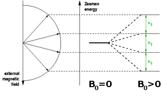
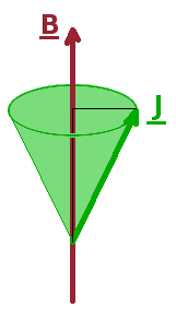
If a spin or other angular momentum is placed in an external magnetic field, it will begin a precession movement around the field axis. If this spin is connected to an electron, this effectively produces an eddy current around the axis of the external field. This current in turn induces another local magnetic field, which acts exactly in the opposite direction of the external field. The net result is the reduction of the external field by a small amount. At the same time, the external field breaks the degeneracy of the states whose angular momentum (and hence magnetic moment) is orientated differently with respect to the field axis. This Zeeman splitting is proportional to the size of the field: $$\hat{H}_{\textrm Zeeman}\propto\vec{J}\cdot\vec{B}\qquad.$$ Therefore, the distance between the Zeeman levels and thus the frequency of electromagnetic radiation which can trigger transitions between them is also proportional to the field.
Since the local electronic environment reduces the effective magnetic field due to its diamagnetism, there is a chemical shift of the frequency of such transitions between Zeeman levels. This is a small effect, of the order of tens of parts per million (ppm), at frequencies of the order of tens or hundreds of MHz depending on the type of nucleus used. Good nuclei have a nuclear spin, high isotope abundance and concentration in the sample and a large gyromagnetic ratio. $\mathrm{^{29}Si}$ and $\mathrm{^{27}Al}$ are frequently used for studies of inorganic materials containing these elements, although the most common NMR nuclei are $\mathrm{^1H}$, $\mathrm{^2D}$ and $\mathrm{^{13}C}$, mostly for studies of organic compounds including polymers.
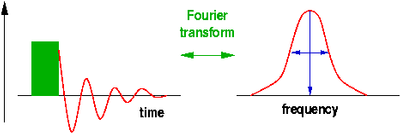
The quantum $h\nu$ needed to trigger a transition of a spin (magnetic moment) from one Zeeman level to another is provided in the form of radiofrequency (rf) electromagnetic radiation induced by a pulsed rf current in a coil surrounding the sample and placed, along with it, into the external magnetic field. During the rf pulse, the Boltzmann populations of the Zeeman levels are being disrupted. When a spin is excited, the orientation of its magnetic moment reverses, so the vector sum of all the magnetic moments, the macroscopic magnetisation of the sample rotates away from the direction of the magnetic field. After the end of the pulse, this process is reversed, the sample equilibrates back to a Boltzmann distribution, and the change of the magnetisation induces a current in the same coil that was previously used for the excitation. The frequency components of this current are analysed using Fourier transformation to reveal the NMR spectrum. The position of the line, the chemical shift, indicates the local electron density surrounding the probe nucleus. This can be used to differentiate co-ordination environments, e.g. a tetrahedral environment generally has a higher electron density (and thus chemical shift) than an octahedral environment, where the nearest neighbours tend to be further away. The technique is sensitive enough to distinguish environments which only differ in their second co-ordination sphere. The width of the peak, at least if ionic mobility can be neglected, is determined by the distribution of environments and is therefore indicative of the amount of disorder in the structure.
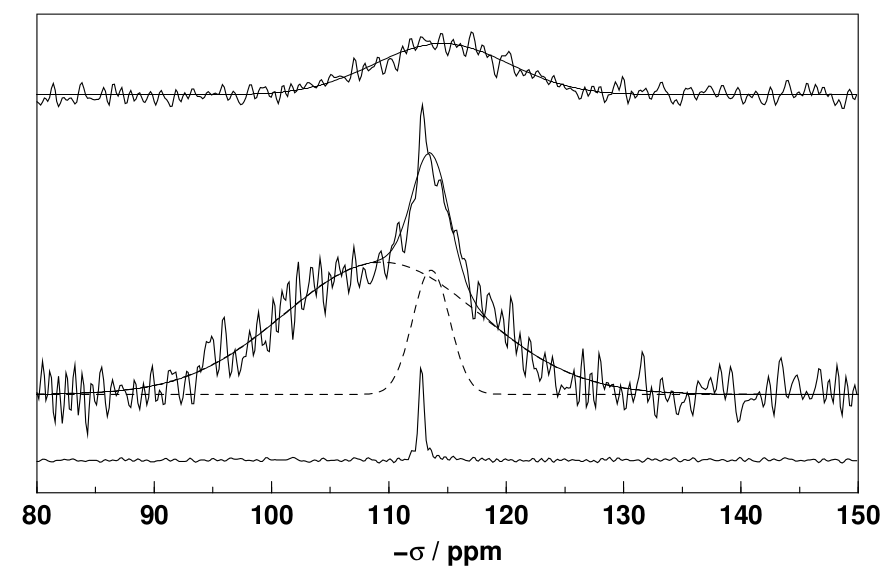
Returning to the nearly fully amorphised sample from the case study, we can compare its $\mathrm{^{29}Si}$ NMR spectrum with that of a melted silica glass (top row) and crystalline quartz (bottom row). It is evident that a wide and a narrower Gaussian line are superimposed on one another. Both are broader (by fwhm) than the corresponding lines in the crystalline and amorphous reference samples, indicating that both environments in the ball-milled sample are more distorted and thus subject to more line broadening than the reference materials. It can also be seen that the peaks are shifted to the left, to larger (more negative) chemical shifts, suggesting that the electron density surrounding the silicon atoms is higher - in line with a sample that has been subject to large compressive stresses during the ball milling experiment.

The advantage of NMR over diffraction when it comes to amorphous structures is that it maps the average environment surrounding a species of atom in the sample, establishing co-ordination numbers and polyhedra via the peak position, and the extent of dihedral angle disorder via the peak width. However, scattering techniques are also capable of capturing this information. This kind of information about non-periodic structures is contained in the diffuse scattering component rather than in the Bragg peaks. It maps the distribution of atoms surrounding a central atom, the pair distribution function (PDF), $g(r)$. The atoms surrounding a central atom are arranged in co-ordination spheres, and the number of atoms in a narrow spherical shell can be counted as the shell radius increases. Even for a crystal structure, this produces a complicated function of the radial distance from the central atom with many peaks and troughs. The number of atoms of type $l$ surrounding a central atom of type $k$ is $$n_{kl}(r)=4\pi r^2\rho_lg_{kl}(r)\qquad,$$ where $\rho_l$ is the number density of atoms of type $l$ in the sample and $g_{kl}(r)$ is the pair distribution function of $k-l$ pairs in the sample. The factor $4\pi r^2$ is the rate at which the volume of a spherical shell increases as the radial distance increases. The PDF remains at 0 up to the bond length of a chemical bond of the pair of atoms, it then varies according to the distribution of $l$ atoms as seen from the $k$ atom at the centre before approaching 1 in the limit of large radial distances, where we just see the average structure.
In a binary (AB) compound, three different PDFs exist: one for pairs of two A atoms, $g_{AA}(r)$, one for pairs of two B atoms, $g_{BB}(r)$, and one for mixed pairs, $g_{AB}(r)$. It is impossible to measure these independently using scattering techniques; a scattering experiment always sees a superposition of all three PDFs. For compounds with more elements, the number of contributing PDFs grows rapidly. What we can work out using scattering techniques is the experimental radial distribution function (RDF), $G(r)$, $$G(r)=\sum_{\textrm{k,l pairs}}c_kc_lb_kb_l[g_{kl}(r)-1]\qquad,$$ which is a weighted sum of all PDFs in the sample, weighted by the concentrations and scattering efficiencies (scattering lengths or atomic form factor) of the different atom types in each pair. The term $-1$ serves to shift all contributing PDFs in such a way that they oscillate around a value of zero rather than one, which makes RDFs from samples with different numbers of elements comparable - otherwise the large-$r$ tails of the contributing PDFs would add up. Since scattering events occur in reciprocal space, the direct-space radial distribution function is accessed via Fourier transformation of the structure factor, $S(q)$, i.e. the scattering pattern normalised to the incident flux from the source: $$G(r)=\frac{2}{\pi}\int_0^{\infty}q[S(q)-1]\sin{(qr)}{\rm d}q\qquad.$$
As is always the case with Fourier transforms, broad features in the reciprocal domain transform into sharp features in the direct domain and vice versa. Therefore, we can expect long-range correlations typical of crystal structures to produce very sharp Bragg diffraction peaks, while short-range order in both crystalline and amorphous samples will result in oscillations over a large $q$ range in reciprocal space. The combination of this diffuse scattering and Bragg diffraction is known as total scattering.
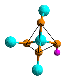
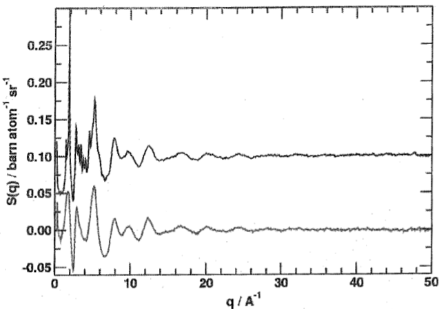
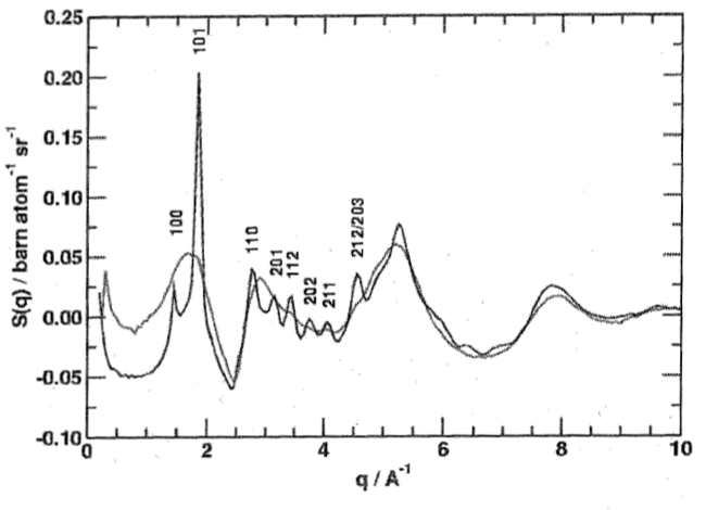
The low-$q$ part of the neutron scattering pattern of nano-crystalline and amorphised $\mathrm{SiO_2}$ demonstrates this: The oscillations in both patterns are largely identical, indicating that the short-range order is the same in both forms, i.e. they consist of the same $\mathrm{SiO_4}$ tetrahedra. However, the nano-crystalline form also has sharp Bragg peaks which can be indexed as usual in Bragg diffraction. To translate the position of the Bragg peaks from the scattering angle ($2\theta$) units typical of diffraction into the momentum transfer ($q$) units used in total scattering, we can use the formula $$q=\frac{4\pi}{\lambda}\sin\left(\frac{\theta}{2}\right)\qquad,$$ which contains the wavelength $\lambda$ of the incident radiation.
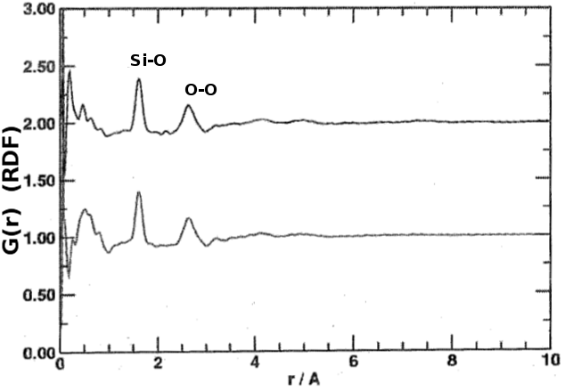
The short-range configuration is revealed by Fourier-transforming the scattering patterns. The Fig. shows the RDFs of the amorphous and nano-crystalline samples, which are practically identical. The atomic distances of both nearest neighbours and next-nearest neighbours are evident at about 1.6 and 2.6 Ångströms, respectively. Provided the data have been properly normalised, the co-ordination numbers can be determined by integrating the peaks. From the co-ordination number and the next-nearest neighbour distance, the shape of the co-ordination polyhedron can be deduced, and the width of the peaks reflects the dihedral angle disorder, the latter being the most significant difference between the short-range order of crystals and glasses of the same composition.
L Cormier, PH Gaskell, G Calas, AK Soper
Medium-range order around titanium in a silicate glass
studied by neutron diffraction with isotopic substitution
Phys Rev B 58 (1998) 11322
While total scattering makes it possible to derive the local structure of solids (and indeed liquids), it suffers from the problem that the information contained in the scattering pattern is a superposition of the environments of all the different atom types present. It can be difficult to disentangle this information because the correlation peaks from different atom pairs in the RDF may overlap. While this can be resolved by modelling (fitting a structural model to the data by computer simulation), it is possible to obtain experimental data with chemical specificity by contrast variation, i.e. by changing the scattering probability for a certain element in the sample. There are a number of different methods which achieve this. In neutron scattering, it is possible to exploit the fact that the scattering length, $b$, is a property of the nucleus and will therefore be different for different isotopes of the same element. Therefore, isotopic substitution (enrichment, labelling) of the sample will give the interactions of a particular element either a larger or a smaller weight compared to an otherwise identical sample with a natural isotope ratio. In x-ray scattering, there is no isotope effect but it is possible to change the atomic form factor due to its energy dependence in the vicinity of an absorption edge of an element - we will see an example of this anomalous scattering technique on the next page.
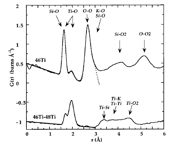
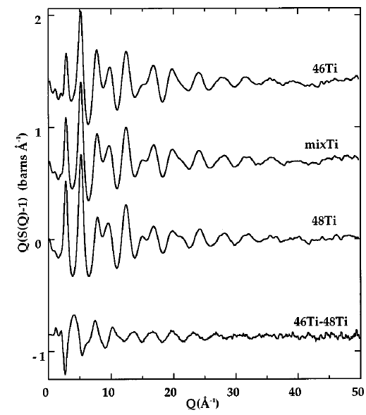
The Fig. above shows the scattering patterns of three potassium titanium silicate glasses with identical chemical composition but different isotopic composition with respect to titanium. It is clear that the structure is the same as the peaks and troughs of the curves appear in the same places. However, the amplitudes of certain features differ between the samples. This is due to the different scattering lengths of the two titanium isotopes present, and the differences can be quantified by subtracting one pattern from another, as shown in the bottom trace. If measurements are made with three different isotope ratios carefully chosen in such a way that they differ by the same amount in the average scattering length ($b_1-b_2=b_2-b_3$), the difference signal contains exclusively the correlations between titanium atoms. Provided that an element has at least two isotopes that have a reasonable neutron scattering cross section, the partial scattering function can be determined for this element, containing information exclusively relating to atoms of the labelled element. Like the total scattering function, the partial scattering function can be Fourier-transformed in order to reveal the real-space distribution of atoms. In the case of a partial scattering function, this leads to the differential pair distribution functions pertaining specifically to the labelled element, i.e. the correlations between the positions of atoms of this species. The Fig. shows the differential PDF for titanium (bottom) and the full RDF of one of the samples (top), which contains the information from all species superimposed on each other, including the relatively small contribution from titanium.
We have seen here that diffuse scattering contains important structural information beyond the periodicity of the crystal lattice, in particular about characteristic lengths within co-ordination environments on the atomic scale. However, diffuse scattering can also tell us a lot about the larger scale and the morphology of a material. Scattering techniques focussing on this aspect of the structure are known as small-angle scattering techniques.