
Phonons are a crystal's way of storing thermal energy. Each chemical bond is treated as an oscillator (effectively a spring) whose fundamental frequency is determined by the elastic constant (spring constant) and the masses of the attached atoms. However, since no bond is isolated but rather part of a crystal lattice, oscillations do not occur on individual bonds. Instead, vibration modes are excited along certain lattice directions.
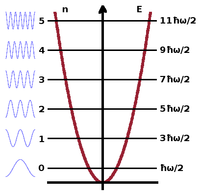
As long as the oscillations can be treated as elastic, i.e. Hooke's law can be taken to be valid, the quantum-mechanical harmonic oscillator model determines the energy levels of a particular mode and its harmonics: $$E_n=\left(n+\frac{1}{2}\right)\hbar\omega\qquad,$$ where $n$ is the vibrational quantum number. The ½ term represents the zero-point energy corresponding to the fundamental mode and is a consequence of the uncertainty principle. The Boltzmann distribution allows us to determine the relative population of each energy level as a function of temperature: $$\frac{N_n}{N}=\frac{\exp{\left(\frac{-n\hbar\omega}{k_BT}\right)}}{\sum_s\exp{\left(\frac{-s\hbar\omega}{k_BT}\right)}}$$ We can use this to calculate the average quantum number, $\langle n\rangle$, i.e. the number of phonons exciting a particular mode. The average quantum number is equal to the weighted sum of the quantum numbers of each level $s$, where each level is weighted with its relative population:
$$\langle n\rangle=\sum_ss\frac{N_s}{\sum_sN_s}\quad\color{grey}{=0\frac{N_0}{N_0+N_1+N_2+\dots}+1\frac{N_1}{N_0+N_1+N_2+\dots}+2\frac{N_2}{N_0+N_1+N_2+\dots}+\dots}$$
The first three terms of the sum are shown in grey to illustrate the workings of the summation. Since the partition function in the denominator is the same for each term of the outer sum, we can move the outer sum sign into the numerator - again, the first terms of the ratio of sums are shown in grey to demonstrate the validity of this move:
$$\qquad=\frac{\sum_ss\exp{\left(\frac{-s\hbar\omega}{k_BT}\right)}}{\sum_s\exp{\left(\frac{-s\hbar\omega}{k_BT}\right)}} \quad\color{grey}{=\frac{0N_0+1N_1+2N_2+\dots}{N_0+N_1+N_2+\dots}}\qquad.$$
By taking the factor $s$ out of the exponential function based on the fact that an exponent comprising a product is equivalent to applying the two powers sequentially, we can re-write the ratio as
$$\qquad=\frac{\sum_ss\left(\exp{\left(\frac{-\hbar\omega}{k_BT}\right)}\right)^s}{\sum_s\left(\exp{\left(\frac{-\hbar\omega}{k_BT}\right)}\right)^s} =\frac{\bbox[lightblue]{\sum_ssx^s}}{\bbox[lightgreen]{\sum_sx^s}}\qquad\color{grey}{\left[a^{bc}=(a^b)^c\right]},$$
using $x=\exp{\left(\frac{-\hbar\omega}{k_BT}\right)}$ as temporary shorthand. This emphasises that the denominator is the geometric series, which converges to $$\bbox[lightgreen]{\sum_sx^s}=\frac{1}{1-x}\qquad(\textrm{for}\,x\lt 1)\qquad.$$ The numerator is equal to the product of $x$ and the derivative of the geometric series:
$$\bbox[lightblue]{\sum_ssx^s}=x\frac{{\rm d}}{{\rm d}x}\sum_sx^s=x\frac{{\rm d}}{{\rm d}x}\frac{1}{1-x}=x\left(-\frac{1}{(1-x)^2}\right)\frac{{\rm d}}{{\rm d}x}(1-x)=\frac{x}{(1-x)^2}\qquad,$$
as can be seen by comparing the first few terms of both sums:
$$\color{grey}{0x^0+1x^1+2x^2+\dots=x\frac{{\rm d}}{{\rm d}x}(x^0+x^1+x^2+\dots)}\qquad.$$
These terms can be substituted for the sums in the denominator and numerator, respectively. Since they are quite similar, they simplify nicely:
$$\langle n\rangle=\frac{\bbox[lightblue]{\sum_ssx^s}}{\bbox[lightgreen]{\sum_sx^s}} =\frac{\frac{x}{(1-x)^2}}{\frac{1}{1-x}} =\frac{x}{1-x} =\frac{\exp{\left(\frac{-\hbar\omega}{k_BT}\right)}}{1-\exp{\left(\frac{-\hbar\omega}{k_BT}\right)}}\qquad.$$
We can further simplify by expanding the fraction by the positive counterpart of the exponential:
$$\qquad=\frac{\exp{\left(\frac{-\hbar\omega}{k_BT}\right)}}{1-\exp{\left(\frac{-\hbar\omega}{k_BT}\right)}}\cdot\frac{\exp{\left(\frac{\hbar\omega}{k_BT}\right)}}{\exp{\left(\frac{\hbar\omega}{k_BT}\right)}} =\frac{1}{\exp{\left(\frac{\hbar\omega}{k_BT}\right)}-1}\qquad,$$
leaving a function with a single positive exponential. This form is known as the Planck distribution. With it, it becomes possible to calculate the average quantum number of a system of oscillators without having to consider each individual energy level individually; only the temperature and the fundamental frequency have to be known.
The total vibrational energy of the lattice can then be calculated by substituting the average quantum number into the formula for the energy of a specific level of the harmonic oscillator:
$$E_{vib}=\sum_i\left(\langle n_i\rangle+\frac{1}{2}\right)\hbar\omega_i\approx\sum_i\langle n_i\rangle\hbar\omega_i =\sum_i\frac{\hbar\omega_i}{\exp{\left(\frac{\hbar\omega_i}{k_BT}\right)}-1}\qquad.$$
The sum in this formula is over the different modes (oscillations having different wave vectors) and polarisations (longitudinal and two transversal) rather than over different energy levels of the same mode (as the average quantum number takes care of that). Since there are many modes in a crystal, we can substitute the sum with an integral: $$E_{vib}=\int D(\omega)\frac{\hbar\omega}{\exp{\left(\frac{\hbar\omega}{k_BT}\right)}-1}{\rm d}\omega\qquad.$$ In it, the density of states, $D(\omega)$, describes how many different modes exist in a frequency band ${\rm d}\omega$. The energy formula in this form is reasonably general - the only severe assumption made is that the oscillators are harmonic, i.e. operate in an elastic regime according to Hooke's law. Beyond that, the particular form chosen for the density of states reflects our model of the crystal and therefore contains our understanding of the vibrational properties of the crystal. We will be looking at two relatively simple models which can be solved analytically in the next two boxes on this page, followed by a more general approach requiring numerical solution strategies.
Once we have determined the vibrational energy and its dependence on the temperature, we can calculate the vibrational heat capacity, $c_{vib}$, by differentiating the energy with respect to temperature: $$c_{vib}=\frac{{\rm d}E_{vib}}{{\rm d}T} =\frac{{\rm d}}{{\rm d}T}\int D(\omega)\frac{\hbar\omega}{\exp{\left(\frac{\hbar\omega}{k_BT}\right)}-1}{\rm d}\omega$$ As the integral and the derivative in this equation relate to different variables (frequency and temperature, respectively), we can swap them around. Since the density of states (unlike their population!) does not change with temperature, it can be taken outside the derivative along the other factors independent of temperature: $$\qquad=\int D(\omega)\hbar\omega\frac{{\rm d}}{{\rm d}T}\left(\frac{1}{\exp{\left(\frac{\hbar\omega}{k_BT}\right)}-1}\right){\rm d}\omega\qquad.$$ Differentiating involves applying the chain rule twice:
$$\qquad=\int D(\omega)\hbar\omega\left(-\frac{1}{\left(\exp{\left(\frac{\hbar\omega}{k_BT}\right)}-1\right)^2}\right)\frac{{\rm d}}{{\rm d}T}\left(\exp{\left(\frac{\hbar\omega}{k_BT}\right)}-1\right){\rm d}\omega$$ $$\qquad=\int D(\omega)\hbar\omega\left(-\frac{1}{\left(\exp{\left(\frac{\hbar\omega}{k_BT}\right)}-1\right)^2}\right)\exp{\left(\frac{\hbar\omega}{k_BT}\right)}\frac{\hbar\omega}{k_B}\left(-\frac{1}{T^2}\right){\rm d}\omega\qquad.$$
With some tidying up, we get a formula for the heat capacity within the same limits of applicability as for the vibrational energy:
$$c_{vib}=\int D(\omega)\frac{\hbar^2\omega^2\exp{\left(\frac{\hbar\omega}{k_BT}\right)}}{k_BT^2\left(\exp{\left(\frac{\hbar\omega}{k_BT}\right)}-1\right)^2}{\rm d}\omega=k_B\int D(\omega)\frac{x^2{\rm e}^x}{({\rm e}^x-1)^2}{\rm d}\omega\qquad\left(\textrm{where}\,x=\frac{\hbar\omega}{k_BT}\right)\qquad.$$
The subsitution $x$ is made frequently in the literature for brevity's sake.
In order to calculate the vibrational heat capacity of a solid we have to find a suitable model representing the solid and infer the appropriate density of states from it. A simple model for this purpose is the Einstein model. It is based on the assumption that all oscillators have the same frequency $\omega_0$. The density of states is then simply $$D(\omega)=3N\delta(\omega-\omega_0)\qquad,$$ where the delta function rejects all frequencies that are not equal to $\omega_0$. The factor $3N$ arises from the fact that each of the $N$ atoms in the crystal has three degrees of freedom of motion. The resulting vibrational energy and heat capacity therefore become
$$E_{vib}=\int D(\omega)\frac{\hbar\omega}{\exp{\left(\frac{\hbar\omega}{k_BT}\right)}-1}{\rm d}\omega=\frac{3N\hbar\omega_0}{\exp{\left(\frac{\hbar\omega_0}{k_BT}\right)}-1}\qquad,\,\textrm{and}$$ $$c_{vib}=\int D(\omega)\frac{\hbar^2\omega^2\exp{\left(\frac{\hbar\omega}{k_BT}\right)}}{k_BT^2\left(\exp{\left(\frac{\hbar\omega}{k_BT}\right)}-1\right)^2}{\rm d}\omega=\frac{3N\hbar^2\omega_0^2\exp{\left(\frac{\hbar\omega_0}{k_BT}\right)}}{k_BT^2\left(\exp{\left(\frac{\hbar\omega_0}{k_BT}\right)}-1\right)^2}\qquad,$$
respectively.
To assess whether this rather simple model produces realistic results, we investigate the high- and low-temperature limits of the heat capacity. In the high-temperature limit, we expect the heat capacity to approach the value of 3R (where R is the gas constant): $$\lim_{T\to\infty}c_{vib}=3N_Ak_B=3R\qquad.$$ This is known as the rule of Dulong and Petit and agrees quite well with experimental observations. It is based on the equipartition theorem of thermodynamics, which assigns $\frac{1}{2}k_BT$ per degree of freedom to both the potential and kinetic energies of an atom or molecule.
Unfortunately, in the case of the Einstein model, it is not immediately clear what the high-temperature limit might be as the different temperature-dependent terms pull $c_{vib}$ in different directions: $$\lim_{T\to\infty}c_{vib}=\lim_{T\to\infty}\frac{3N\hbar^2\omega_0^2\color{red}{\cancel{\color{black}{\exp{\left(\frac{\hbar\omega_0}{k_BT}\right)}}}^1}}{k_B\color{red}{\cancel{\color{black}{T^2}}^{\infty}}\color{red}{\cancel{\color{black}{\left(\exp{\left(\frac{\hbar\omega_0}{k_BT}\right)}-1\right)^2}}^0}}\qquad.$$ We can use de l'Hôpital's rule to resolve this problem. It states that the limit of the ratio of two functions is equal to the limit of their derivatives (as long as both numerator and denominator are differentiable): $$\lim_{x\to x_0}\frac{f(x)}{g(x)}=\lim_{x\to x_0}\frac{\quad\frac{{\rm d}f(x)}{{\rm dx}}\quad}{\frac{{\rm d}g(x)}{{\rm d}x}}\qquad.$$ If we bring the $T^2$ factor onto the numerator, both numerator and denominator approach zero as the temperature goes to infinity, and we can use de l'Hôpital's rule and differentiate both separately:
$$\lim_{T\to\infty}c_{vib}=\lim_{T\to\infty}\frac{\frac{3N\hbar^2\omega_0^2}{k_BT^2}\exp{\left(\frac{\hbar\omega_0}{k_BT}\right)}}{\left(\exp{\left(\frac{\hbar\omega_0}{k_BT}\right)}-1\right)^2}=\lim_{T\to\infty}\frac{\frac{{\rm d}}{{\rm d}T}\left(\frac{3N\hbar^2\omega_0^2}{k_BT^2}\exp{\left(\frac{\hbar\omega_0}{k_BT}\right)}\right)}{\frac{{\rm d}}{{\rm d}T}\left(\left(\exp{\left(\frac{\hbar\omega_0}{k_BT}\right)}-1\right)^2\right)}\qquad.$$
The numerator takes a combination of the chain rule and the product rule to solve, the denominator requires two consecutive applications of the chain rule:
$$\qquad=\lim_{T\to\infty}\frac {\frac{3N\hbar^2\omega_0^2}{k_B}\left[\left(-\frac{2}{T^3}\right)\exp{\left(\frac{\hbar\omega_0}{k_BT}\right)}+\frac{1}{T^2}\frac{\hbar\omega_0}{k_B}\left(-\frac{1}{T^2}\right)\exp{\left(\frac{\hbar\omega_0}{k_BT}\right)}\right]} {2\left(\exp{\left(\frac{\hbar\omega_0}{k_BT}\right)}-1\right)\left(-\frac{\hbar\omega_0}{k_BT^2}\right)\exp{\left(\frac{\hbar\omega_0}{k_BT}\right)}}$$
After tidying up, we are still left with a ratio of two functions which both approach zero in the high-temperature limit. At least, the temperature dependence has simplified, so we should be able to find the limit by applying de l'Hôpital's rule again:
$$\qquad=\lim_{T\to\infty}\frac {\frac{3N\hbar\omega_0}{T}\left(1+\frac{\hbar\omega_0}{2k_BT}\right)} {\exp{\left(\frac{\hbar\omega_0}{k_BT}\right)}-1} =\lim_{T\to\infty}\frac {\frac{{\rm d}}{{\rm d}T}\left[\frac{3N\hbar\omega_0}{T}\left(1+\frac{\hbar\omega_0}{2k_BT}\right)\right]} {\frac{{\rm d}}{{\rm d}T}\left(\exp{\left(\frac{\hbar\omega_0}{k_BT}\right)}-1\right)}\qquad.$$
This takes another application of the product and chain rule, respectively:
$$\qquad=\lim_{T\to\infty}\frac {3N\hbar\omega_0\left[\left(-\frac{1}{T^2}\right)\left(1+\frac{\hbar\omega_0}{2k_BT}\right)+\frac{1}{T}\frac{\hbar\omega_0}{2k_B}\left(-\frac{1}{T^2}\right)\right]} {\frac{\hbar\omega_0}{k_B}\left(-\frac{1}{T^2}\right)\exp{\left(\frac{\hbar\omega_0}{k_BT}\right)}}\qquad,$$
and after tidying up, we finally have a ratio of finite values in the high-temperature limit:
$$\qquad=\lim_{T\to\infty}\frac {3N\hbar\omega_0\left(-\frac{1}{T^2}-\frac{\hbar\omega_0}{2k_BT^3}-\frac{\hbar\omega_0}{2k_BT^3}\right)} {-\frac{\hbar\omega_0}{k_BT^2}\exp{\left(\frac{\hbar\omega_0}{k_BT}\right)}} =\lim_{T\to\infty}3Nk_B\frac{1+\color{red}{\cancel{\color{black}{\frac{\hbar\omega_0}{k_BT}}}^0}}{\color{red}{\cancel{\color{black}{\exp{\left(\frac{\hbar\omega_0}{k_BT}\right)}}}^1}}=3Nk_B$$
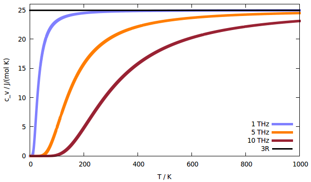
Even better, the predicted limit matches the expectation according to Dulong and Petit! The plot of the Einstein heat capacity above shows that the Dulong-Petit limit is approached faster at relatively low frequencies than at higher ones. Note that even a frequency considered "low" in phonon terms is typically in the low THz range.
Clearly, the Einstein model is spot on in the high-temperature limit, despite its simplicity. What about the low-temperature limit, though? In this case, we're not just looking at the value of the heat capacity in the limit of $T\to 0$ but rather at the shape of the curve as it begins to rise. By inspecting the order of magnitude of the argument of the exponential, we find that $$O\left(\frac{\hbar\omega_0}{k_BT}\right)=\frac{10^{-34}\,2\pi\,10^{12}}{10^{-23}O(T)}\approx\frac{10^2}{O(T)}\qquad,$$ where the $2\pi$ comes from the fact that the formula contains the angular frequency. In the limit of temperatures of no more than a few Kelvins, the argument of the exponential will be of the order of 100, so the exponential will be a very large number, compared to which we can neglect the 1 in the denominator:
$$c_{vib}=\frac{\frac{3N\hbar^2\omega_0^2}{k_BT^2}\exp{\left(\frac{\hbar\omega_0}{k_BT}\right)}}{\left(\exp{\left(\frac{\hbar\omega_0}{k_BT}\right)}\color{red}{\cancel{\color{black}{-1}}}\right)^2}\approx\frac{3N\hbar^2\omega_0^2}{k_BT^2}\exp{\left(-\frac{\hbar\omega_0}{k_BT}\right)}\qquad.$$
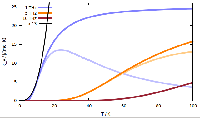
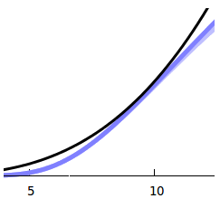
The diagram below shows the behaviour of the Einstein model (bold colours) and its low-temperature approximation (soft colours). The temperature at which the low-temperature approximation deviates from the full model depends on the frequency, but as long as the heat capacity is below R (the gas constant), the approximation is quite good in relation to the model. However, it demonstrates that the Einstein model produces a $T^{-2}{\rm e^{-1/T}}$ dependence. This doesn't reflect the experimentally observed $T^3$ dependence at all. The deviation from the observed relationship is shown magnified in the figure on the right. We have to conclude that the Einstein model is too simplistic to describe low-temperature modes in crystals adequately, even though it is perfectly fine at higher temperatures.
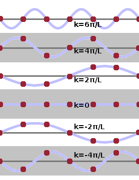
To capture the low-temperature behaviour of the heat capacity correctly, it is necessary to go beyond the simple assumption of the Einstein model that all modes in the crystal have the same fundamental frequency. Instead, we need to identify and count the different modes present based on a model of the crystal structure. Modes are standing waves in the crystal. Therefore, the possible wave numbers for a particular crystallographic orientation are given by $$k=0,\pm\frac{2\pi}{L},\pm\frac{4\pi}{L},\dots,\frac{N\pi}{L}\qquad,$$ where $L$ and $N$ are the size of the grain and the number of atoms along that orientation, respectively. The figure shows the situation for a small crystal six unit cells wide. Oscillations with wave vectors $|k|\gt\frac{N\pi}{L}$ fall outside the Brillouin zone boundary, i.e. they replicate the same atom displacements that are already represented by another, smaller, wavevector. Counting the different wave numbers, it is clear that there is one $k$ value per $\frac{2\pi}{L}$, or, analoguously in 3D, one $k$ per $\left(\frac{2\pi}{L}\right)^3$. To count the total number of modes (wave vectors) contained in the crystal, we need to multiply the number density of modes, $\left(\frac{L}{2\pi}\right)^3$, by the reciprocal space volume taken up by all wave vectors within a sphere of radius $k$: $$N=\left(\frac{L}{2\pi}\right)^3\left(\frac{4}{3}\pi k^3\right)=\frac{Vk^3}{6\pi^2}\qquad,$$ where $V$ is the macroscopic volume of the crystal grain.
The density of states is the derivative of $N$ with respect to frequency - literally how densely the states are spaced along the frequency axis:
$$D(\omega)=\frac{{\rm d}N}{{\rm d}\omega}=\frac{V}{6\pi^2}\frac{{\rm d}}{{\rm d}\omega}k^3=\frac{V}{6\pi^2}3k^2\frac{{\rm d}k}{{\rm d}\omega} =\frac{Vk^2}{2\pi^2}\frac{{\rm d}k}{{\rm d}\omega}\qquad.$$
From this point onward, we need to have a model of the crystal which lets us determine the dispersion relation, $\omega(k)$, from which $\frac{{\rm d}k}{{\rm d}\omega}$ can be calculated.
A relatively simple but analytically solvable model is the Debye model, which assumes that the crystal can be treated as an isotropic elastic medium. Of course this is a rather coarse approximation at least on short length scales, where the periodic pattern of atoms is anything but isotropic. In this model, wave vector and frequency are proportional to one another. The constant of proportionality is the speed of sound, $v_s$, in the medium: $$\omega=v_sk\qquad.$$ This is analogous to the dispersion relation in optics, where the speed of light takes on the role of the speed of sound. With this dispersion relation, we can calculate the Debye density of states: $$D(\omega)=\frac{V\omega^2}{2\pi^2v_s^2}\frac{{\rm d}}{{\rm d}\omega}\frac{\omega}{v_s}=\frac{V\omega^2}{2\pi^2v_s^3}\qquad,$$ and with it the vibrational energy:
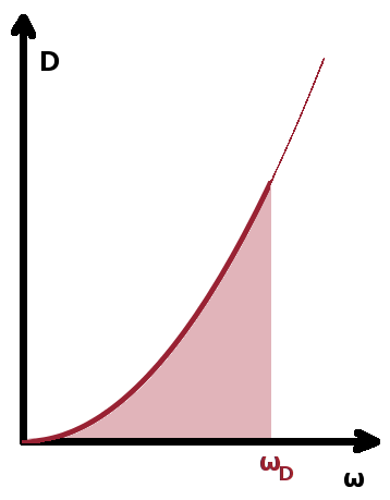
$$E_{vib}=\int D(\omega)\frac{\hbar\omega}{\exp{\left(\frac{\hbar\omega}{k_BT}\right)}-1}{\rm d}\omega =\int_0^{\omega_D}3\frac{V\omega^2}{2\pi^2v_s^3}\frac{\hbar\omega}{\exp{\left(\frac{\hbar\omega}{k_BT}\right)}-1}{\rm d}\omega\qquad.$$
Here, the factor 3 reflects the fact that we have three different polarisations (one longitudinal, two transversal) for each wave vector in a primitive lattice. The upper integration boundary is reduced from infinity to the Debye frequency, the maximum (fundamental) frequency that we can expect in the crystal lattice. This is based on the observation (above) that there is one $k$ per primitive unit cell, producing a total number of modes (as seen above) of $$N=\frac{Vk^3}{6\pi^2}=\frac{V\omega^3}{6\pi^2v_s^3}\qquad.$$ The cutoff frequency is therefore $$\omega_D=v_s\sqrt[3]{\frac{6\pi^2N}{V}}\qquad,$$ and the corresponding cutoff wave vector is $$k_D=\frac{\omega_D}{v_s}=\sqrt[3]{\frac{6\pi^2N}{V}}\qquad.$$ With the substitution
$$x=\frac{\hbar\omega}{k_BT}\quad\Rightarrow\quad \omega=\frac{k_BTx}{\hbar}\quad\Rightarrow\quad \frac{{\rm d}\omega}{{\rm d}x}=\frac{k_BT}{\hbar}\quad\Rightarrow\quad {\rm d}\omega=\frac{k_BT}{\hbar}{\rm d}x\qquad,$$
the vibrational energy becomes
$$E_{vib}=\frac{3V\hbar}{2\pi^2v_s^3}\frac{k_B^3T^3}{\hbar^3}\frac{k_BT}{\hbar}\int_0^{x_D}\frac{x^3}{{\rm e}^x-1}{\rm d}x =\frac{3Vk_B^4T^4}{2\pi^2v_s^3\hbar^3}\int_0^{x_D}\frac{x^3}{{\rm e}^x-1}{\rm d}x\qquad,$$
which is often given in the literature. The Debye temperature, $\Theta_D$, is defined as $$\Theta_D=\frac{\hbar\omega_D}{k_B}=\frac{\hbar v_s}{k_B}\sqrt[3]{\frac{6\pi^2N}{V}}\qquad.$$ It is a material constant which allows us to normalise the temperature dependence of the vibrational properties of different crystals to observe common behaviour on a reduced temperature scale (i.e. when plotting thermodynamic functions against $\frac{T}{\Theta_D}$).
Finally, we can calculate the Debye heat capacity by differentiating the vibrational energy with respect to temperature:
$$c_{vib}=\frac{\partial E_{vib}}{\partial T} =\frac{3V\hbar}{2\pi^2v_s^3}\frac{\partial}{\partial T}\int_0^{\omega_D}\frac{\omega^3}{\exp{\left(\frac{\hbar\omega}{k_BT}\right)}-1}{\rm d}\omega =\frac{3V\hbar}{2\pi^2v_s^3}\int_0^{\omega_D}\omega^3\left(-\frac{1}{\left(\exp{\left(\frac{\hbar\omega}{k_BT}\right)}-1\right)^2}\right)\frac{\hbar\omega}{k_B}\exp{\left(\frac{\hbar\omega}{k_BT}\right)}\left(-\frac{1}{T^2}\right){\rm d}\omega$$ $$\qquad=\frac{3V\hbar^2}{2\pi^2v_s^3k_BT^2}\int_0^{\omega_D}\frac{\omega^4\exp{\left(\frac{\hbar\omega}{k_BT}\right)}}{\left(\exp{\left(\frac{\hbar\omega}{k_BT}\right)}-1\right)^2}{\rm d}\omega\qquad.$$
With the substitutions above, this can be expressed in terms of the Debye temperature as: $$c_{vib}=\frac{9Nk_BT^3}{\Theta_D^3}\int_0^{x_D}\frac{x^4{\rm e}^x}{({\rm e}^x-1)^2}{\rm d}x$$ For very low temperatures, the upper integration boundary $x_D=\frac{\Theta_D}{T}$ approaches infinity, and the infinite integral expands into a convergent series, i.e. it reduces to a constant factor. Therefore, the experimentally observed $T^3$ dependence of the heat capacity at low temperatures is reproduced faithfully by the Debye model.
The Debye model assumes that the phonon density of states follows a parabolic, i.e. monotonously increasing, dependence of the fundamental frequency of lattice oscillations. This is a consequence of the approximation of the crystal lattice as an isotropic medium. Because a crystal lattice is in fact highly anisotropic, with different wave vectors in different crystallographic orientations, the actual density of states is a lot more complex. The Debye model predicts both the high and low temperature limits correctly, but in order to model the rich behaviour of a real crystal in the medium temperature range, it is necessary to establish realistic dispersion relations and determine the actual density of states, via $\frac{{\rm d}k}{{\rm d}\omega}$, from them.
The Debye model describes the heat capacity of solids well in both the low and high temperature limits. However, the assumption made that the medium is isotropic, i.e. that the vibrational states do not depend on the spatial direction of the wave is far too simplistic to describe the rich vibrational properties of real crystals at intermediate temperatures. Phonon spectroscopy produces experimental dispersion relations that show the variation with crystallographic orientation and capture this richness.