
Each state as obtained as a solution of the Schrödinger equation of the hydrogen atom is characterised by a unique combination of the quantum numbers $n$, $l$ and $m$. Each state can be populated by up to two electrons. Even if we reduce the energy of the system to near absolute zero temperature, not all of the electrons converge on the $n=1$ state but remain in higher states because the $n=1$ state can't take more than two electrons. This has led to Pauli's exclusion principle: No two electrons can share the same state (i.e. have the same quantum numbers) at the same time. Therefore, we need another quantum number to distinguish the two electrons sharing the same spatial state $\psi_{n,l,m}$.
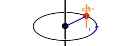
The spin (quantum number), $s$, is similar to $l$ in that it refers to an angular momentum component. It can be visualised as the rotation of the electron, thought of as a particle, around its own axis rather than around the nucleus. However, this description isn't accurate as an electron's behaviour has both aspects of particle (such as scattering) and wave (such as diffraction), and if carried through quantitatively doesn't give accurate results. The value of $s$ is always $s=\frac{1}{2}$ for electrons. Alongside $s$, there is a magnetic spin quantum number, $m_s$, whose possible values are $m_s=\pm\frac{1}{2}$ for electrons. The relationship of $s$ and $m_s$ is the same as that of $l$ and $m$ (the latter often written as $m_l$ to avoid ambiguity if spin is considered). With these additional quantum numbers, we have unique wave functions for single-electron states. These consist of a space function and a spin function: $$\psi_{n,l,m_l,s,m_s}=\psi^{space}_{n,l,m_l}\cdot\psi^{spin}_{s,m_s}\quad.$$ As long as it is clear that we're dealing with electrons (as opposed to other elementary particles), the value of $s$ is fixed to $\frac{1}{2}$, so there is no need to mention it explicitly.
The components of angular momentum are quantised. This applies both to orbital angular momentum (quantum number $l$) and to spin (quantum number $s$).
The uncertainty principle applies to all products of observables whose units combine to [J s] = [kg m2 s-1], i.e. the dimension of Planck's constant. The best-known uncertainty principle is the one linking the uncertainties of position, $x$, and momentum, $p$. There is also an energy-time uncertainty relationship which surfaces when discussing energy bands.
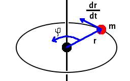
Angular momentum is a vector defined by the cross product $\vec{L}=m\vec{r}\times\frac{{\rm d}\vec{r}}{{\rm d}t}$. Judging by its units, [kg][m]×[m s-1]=[kg m2 s-1], the complementary uncertainty should be dimensionless. It is in fact the uncertainty of the angle of rotation, $\varphi$.
The uncertainty of the angle must be limited to $2\pi$ - the angular momentum has to point somewhere on a circular orbit. Therefore, the uncertainty of the component of the angular momentum perpendicular to the direction of motion must be of the order of Planck's constant. We may therefore conclude that values of $L_z$ are quantised in multiples of $\frac{h}{2\pi}=\hbar$.
There are $2l+1$ possible orientations of the angular momentum, where the $z$ component of the angular momentum is $L_z=-l\hbar, -(l-1)\hbar,$$ \dots, $$(l-1)\hbar, l\hbar$, and two ($2s+1$) possible orientations of the spin of an electron, with $S_z=\pm\frac{\hbar}{2}$. The actual (observable) angular momentum for a state with a quantum number $l$ is $$|\vec{L}|=\sqrt{l(l+1)}\hbar\quad.$$
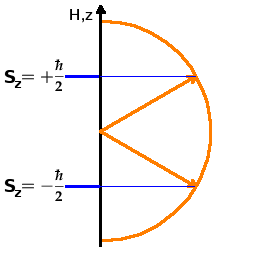
The Fig. shows the situation for the spin: The spin aligns at an angle with the $z$ axis (which could be a preferential axis generated by applying a magnetic field or by a chemical bond). There are two possible orientations (these are often called parallel or up and anti-parallel or down although that's exactly what they are not!). The angle with the $z$ axis is given by the need to distribute the $2l+1$ states uniformly over the whole angular range from the $+z$ to the $-z$ direction. For example, in the case of an $l=1$ angular momentum state, there are three possible orientations, one of which is perpendicular to the $z$ axis, and the other two are 45o off the positive and negative $z$ axis, respectively. In no case is the angular momentum vector exactly (anti-) parallel to the $z$ axis. If it was, we would know both the angular momentum and the angle precisely, which would defy the uncertainty principle. This quantisation of the direction of the angular momentum vector is known as directional quantisation. The different states are differentiated by their $m_l$ or $m_s$ quantum number. In the absence of a directing force (such as an external field or a chemical bond), these states remain degenerate, i.e. their energy is the same. By applying an external field to introduce a preferential axis, the degeneracy can be removed; this is the Zeeman effect.
Notation: $\vec{L}$ is the observable physical quantity, the (orbital) angular momentum vector, $|\vec{L}|$ its absolute magnitude. Lower-case $l$ is the (orbital) angular momentum quantum number, and upper-case $L$ with no embellishments is the combined (orbital) angular momentum quantum number for a group of interacting electrons, which we will encounter later. The same distinction applies to the corresponding spin quantities $\vec{S}$, $|\vec{S}|$, $s$ and $S$. To maximise the confusion, states with $l=0$ are referred to as s-states, as in 1s, 2s etc...
If a system is subject to several angular momenta simultaneously, the resulting net angular momentum depends on how the individual momenta are orientated with respect to each other. The classical treatment produces correct results provided the directional quantisation of each contributing momentum is taken into account.
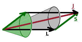
For an electron with orbital angular momentum and spin, this means that we can add the two vectors together - this is the vector model of angular momentum. Because of the uncertainty relation linking angular momentum and angle, the result is that they both precess around the sum vector, which is known as the total angular momentum, $\vec{J}$. As in the case of the constituent angular momenta, there is a total angular momentum quantum number, $j$, whose values range from $|l-s|\cdots l+s$ in integer steps.
Being a charged particle, a moving electron generates a magnetic field. This provides a preferential axis along which the angular momenta of the atom will align. The interaction between the magnetic moment, $\vec{\mu}$, of the electron and the magnetic field $\vec{B}$ results in a perturbation Hamiltonian $\hat{H}'=-\vec{\mu}\cdot\vec{B}$. The energy eigenvalues for this spin-orbit interaction are $$E_{so}\propto\left\langle\frac{1}{r^3}\right\rangle\left\langle\vec{S}\cdot\vec{L}\right\rangle\quad.$$ Here, the expectation value of $r^{-3}$ depends on the quantum number $n$ (as the average size of the electron cloud increases with $n$), and the scalar product of the orbital angular momentum and spin vectors depends on the quantum numbers $l$ and $s$, and we can use the vector model to determine possible values of the product. The constant of proportionality contains all the constituents from the Rydberg constant but goes with $Z^4$, so the spin-orbit interaction becomes much more significant towards the bottom of the periodic table.
The total angular momentum vector is the sum of its two constituent parts: $\vec{J}=\vec{S}+\vec{L}$. Taking the square of that gives $$\left|\vec{J}\right|^2=\left(\vec{S}+\vec{L}\right)^2=\left|\vec{S}\right|^2+\left|\vec{L}\right|^2+2\vec{S}\cdot\vec{L}\quad.$$ By re-arranging for the scalar product, we have $$\vec{S}\cdot\vec{L}=\frac{1}{2}\left(\left|\vec{J}\right|^2-\left|\vec{L}\right|^2-\left|\vec{S}\right|^2\right)\quad.$$ The squares of the angular momenta can be expressed in terms of their respective quantum numbers. As a result the expectation value of the scalar product from the spin-orbit interaction is $$\left\langle\vec{S}\cdot\vec{L}\right\rangle=\frac{1}{2}\left(j(j+1)-l(l+1)-s(s+1)\right)\quad,$$ and the corresponding energy corrections from first-order perturbation theory due to spin-orbit interaction are
$$E_{so}=\frac{\beta}{2}\left(j(j+1)-l(l+1)-s(s+1)\right)\quad,$$
where $\beta$ is the spin-orbit constant combining the constant of proportionality and the $r$-dependence mentioned above.
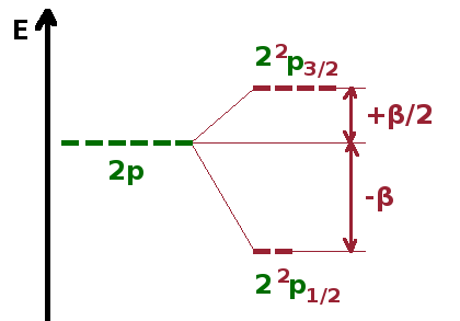
The figure shows the situation for the 2p sub-shell. Taking into account the spin function, there are six individual states characterised by the common quantum numbers $n=2$, $l=1$, $s=\frac{1}{2}$ and distinguished by the quantum numbers $m_l=-1,0,1$ and $m_s=\pm\frac{1}{2}$ - altogether 3x2=6 states.
First we need to work out the possible values of the total angular momentum quantum number $j$:
$j=|l-s|,\cdots,l+s=1-\frac{1}{2},1+\frac{1}{2}=\frac{1}{2},\frac{3}{2}$.
Therefore, the six 2p states split into two sets with different energy:
| $j$ | symbol | multiplicity | $E_{so}$ |
|---|---|---|---|
| $\frac{1}{2}$ | 2 $^2$p$_{\frac{1}{2}}$ | $2\cdot\frac{1}{2}+1=2$ | $\frac{\beta}{2}\left(\frac{1}{2}\cdot\frac{3}{2}-1\cdot 2-\frac{1}{2}\cdot\frac{3}{2}\right)=-\beta$ |
| $\frac{3}{2}$ | 2 $^2$p$_{\frac{3}{2}}$ | $2\cdot\frac{3}{2}+1=4$ | $\frac{\beta}{2}\left(\frac{3}{2}\cdot\frac{5}{2}-1\cdot 2-\frac{1}{2}\cdot\frac{3}{2}\right)=+\frac{\beta}{2}$ |
Here, the multiplicity is the number of degenerate states in each sub-set, i.e. $2j+1$. In this case (and commonly), the splitting is asymmetric, but due to the different multiplicities of each sub-set, the average energy is the same as without spin-orbit interaction: between them, the four $^2$p$_{\frac{3}{2}}$ gain as much energy as the two $^2$p$_{\frac{1}{2}}$ states, combined, lose.
The symbol may look somewhat confusing at first. It begins with the main quantum number (here, 2; omitted if there is no ambiguity) followed by the spectroscopic $l$-symbol (here, p) with two indices. The initial superscript is the spin multiplicity, $2s+1$. For single-electron states, $s$ is always $\frac{1}{2}$, so the spin multiplicity is always 2, so it can be left from the symbol without diminishing the information content. However, we will need this later when interactions between multiple electrons are introduced. Finally, the trailing subscript gives the total angular momentum quantum number $j$ for the sub-set. The quantum numbers make up the full symbol: $n\,^{2s+1}l_j$, where $l$ is represented as a letter (s,p,d,f,...) in spectroscopic notation.
A consequence of this fine structure resulting from spin-orbit interaction is another selection rule for transitions between states subject to this splitting: $\Delta j=0,\pm 1$.
The spin-orbit interaction is a perturbation that occurs even in a simple one-electron hydrogen-like system. As soon as further electrons are added, the picture becomes more complex, and a series of further perturbations is employed to deal with this added complexity. We'll first add a second electron and will later extend the scenario towards atoms further down the periodic table.