
| sub-shell | orbital | spin | total | term |
|---|---|---|---|---|
| 1s | 's' → $l_1=0$ | $s_1=\frac{1}{2}$ | ||
| 2p | 'p' → $l_2=1$ | $s_2=\frac{1}{2}$ | ||
| combi | $\begin{eqnarray}\color{red}{L}&=&|l_1-l_2|\\&=&l_1+l_2\\&=&\color{red}{1}\end{eqnarray}$ | $\begin{eqnarray}\color{red}{S}&=&|s_1-s_2|\\&=&\color{red}{0}\end{eqnarray}$ | $\begin{eqnarray}\color{blue}{J}&=&|L-S|\\&=&L+S\color{blue}{=1}\end{eqnarray}$ | $\bbox[lightgreen]{^1P_1}$ |
| $\begin{eqnarray}\color{red}{S}&=&s_1+s_2\\&=&\color{red}{1}\end{eqnarray}$ | $\color{blue}{J=}|L-S|\color{blue}{=0}$ | $\bbox[lightgreen]{^3P_0}$ | ||
| $\color{blue}{J=}|L-S|+1\color{blue}{=1}$ | $\bbox[lightgreen]{^3P_1}$ | |||
| $\color{blue}{J=}L+S\color{blue}{=2}$ | $\bbox[lightgreen]{^3P_2}$ |
The various orientations of orbital angular momentum and spin give rise to the fine structure of atomic spectra. This is known as spin-orbit coupling or LS coupling since the total orbital angular momentum, $L$, of a group of electrons interacts with the total spin, $S$, of that group of electrons, following the vector model of angular momentum. We've already seen this for hydrogen and for helium. The table recapitulates the situation for an excited helium atom in the 1s 2p configuration. To derive the term symbols for the different spin-orbit states, we first need to calculate the total orbital angular momentum and total spin from those of the individual electrons, respectively (shown by column, in red). Then $L$ and $S$ are combined to find the total angular momentum of this group of electrons, $J$ (shown by row, in blue). The possible combinations for $L$, $S$ and $J$ according to the vector model are given by the Clebsch-Gordan sequences:
$$\begin{eqnarray} L&=&|l_1-l_2|\cdots l_1+l_2\qquad\textrm{(in integer steps)}\\ S&=&|s_1-s_2|\cdots s_1+s_2\qquad\textrm{(in integer steps)}\\ J&=&|L-S|\cdots L+S\qquad\textrm{(in integer steps)} \end{eqnarray}$$
The term symbols are then composed by writing the total orbital angular momentum, $L$, in spectroscopic notation (S,P,D,F,... - capitalised, since this refers to the total orbital angular momentum of a group of electrons) with the total angular momentum, $J$, as a subscript. Finally, the spin multiplicity, $2S+1$, is calculated from the total spin and attached to the term symbol as a leading superscript. The term symbols for all four terms in the 1s 2p configuration are shown in green in the table above. In this case, there is a singlet state ($^1P_1$) and a triplet of states ($^3P_0$, $^3P_1$, $^3P_2$). In almost all cases, the spin multiplicity indicates how many states there are in each group (see below for an exception).
| sub-shell | orbital | spin | |
|---|---|---|---|
| 2p | 'p' → $l_1=1$ | $s_1=\frac{1}{2}$ | |
| 3p | 'p' → $l_2=1$ | $s_2=\frac{1}{2}$ | |
| combi | $\color{red}{L=}|l_1-l_2|\color{red}{=0}$ | $\color{red}{S=}|s_1-s_2|\color{red}{=0}$ | |
| $\color{red}{L=}|l_1-l_2|+1\color{red}{=1}$ | $\color{red}{S=}s_1+s_2\color{red}{=1}$ | ||
| $\color{red}{L=}l_1+l_2\color{red}{=2}$ |
| L→ S↴ | 0→'S' | 1→'P' | 2→'D' |
|---|---|---|---|
| 0 | $\begin{eqnarray}\color{blue}{J}&=&|L-S|\\&=&L+S\\&=&\color{blue}{0}\,\rightarrow\,\bbox[lightgreen]{^1S_0}\end{eqnarray}$ | $\begin{eqnarray}\color{blue}{J}&=&|L-S|\\&=&L+S\\&=&\color{blue}{1}\,\rightarrow\,\bbox[lightgreen]{^1P_1}\end{eqnarray}$ | $\begin{eqnarray}\color{blue}{J}&=&|L-S|\\&=&L+S\\&=&\color{blue}{2}\,\rightarrow\,\bbox[lightgreen]{^1D_2}\end{eqnarray}$ |
| 1 | $\begin{eqnarray}\color{blue}{J}&=&|L-S|\\&=&L+S\\&=&\color{blue}{1}\,\rightarrow\,\bbox[lightgreen]{^3S_1}\end{eqnarray}$ | $\begin{eqnarray}\color{blue}{J}&=&|L-S|\\&=&\color{blue}{0}\,\rightarrow\,\bbox[lightgreen]{^3P_0}\end{eqnarray}$ | $\begin{eqnarray}\color{blue}{J}&=&|L-S|\\&=&\color{blue}{1}\,\rightarrow\,\bbox[lightgreen]{^3D_1}\end{eqnarray}$ |
| $\begin{eqnarray}\color{blue}{J}&=&|L-S|+1\\&=&\color{blue}{1}\,\rightarrow\,\bbox[lightgreen]{^3P_1}\end{eqnarray}$ | $\begin{eqnarray}\color{blue}{J}&=&|L-S|+1\\&=&\color{blue}{2}\,\rightarrow\,\bbox[lightgreen]{^3D_2}\end{eqnarray}$ | ||
| $\begin{eqnarray}\color{blue}{J}&=&L+S\\&=&\color{blue}{2}\,\rightarrow\,\bbox[lightgreen]{^3P_2}\end{eqnarray}$ | $\begin{eqnarray}\color{blue}{J}&=&L+S\\&=&\color{blue}{3}\,\rightarrow\,\bbox[lightgreen]{^3D_3}\end{eqnarray}$ |
In principle, any other electron configuration can be treated in exactly the same way, although the number of different terms can become quite large. The two tables to the right show a simple example of a configuration with two valence electrons, 2p 3p.
Again, the total orbital angular momentum and the total spin are calculated from those of the individual electrons. In this case, the Clebsch-Gordan sequence produces three possible values for $L$ rather than just one. Spin-wise, the situation is the same for any two-electron configuration since the spin of a single electron is always $s=\frac{1}{2}$. We then have to look at all possible permutations of the total orbital angular momenta and the total spin, as shown in the second table on the right. For each permutation, we calculate the total angular momentum, $J$, and work out the term symbol as before. There are three separate singlets, two proper triplets consisting of three states each, and one additional "triplet" state, $^3S_1$. This is an exception to the rule that the multiplicity indicates the number of states in a particular group of terms - the reason this "triplet" has only one member is the fact that the Clebsch-Gordon sequence uses the magnitude of the difference of $L$ and $S$ and thus $|L-S|$ and $L+S$ are the same in this case.
The energies of the different terms depend on the direct and exchange integrals, as we have seen in the case of helium. In principle these can be calculated numerically for all terms using perturbation theory. However, if all we need to know is the configuration of the ground state, Hund's rules can predict which term is populated in the ground state for each configuration without the need to calculate any energies: The term with the lowest energy is the one with the highest $S$. If there are several of those, then the one with the highest $L$ will have the lowest energy. If there are still several, the lowest-energy term will be the one with the lowest $J$. Therefore, from the table above, the term at the bottom of the splitting will be $^3D_1$.
Since perturbation theory is based on making small changes to known systems, perturbations must be applied in the correct order, i.e. in order of decreasing severity. The fine structure (exchange integral) and the residual electrostatic interaction are of comparable size but depend differently on the atom number $Z$. The fine structure splitting increases with $Z^2$, while the residual electrostatic interaction rises only gradually with $Z$. For light elements, near the top of the periodic table, $\hat{H}_{re}$ dominates and has to be applied first, but for heavier elements, this is less clear-cut, and a transition to a different spin-orbit coupling regime, jj coupling occurs as a consequence.
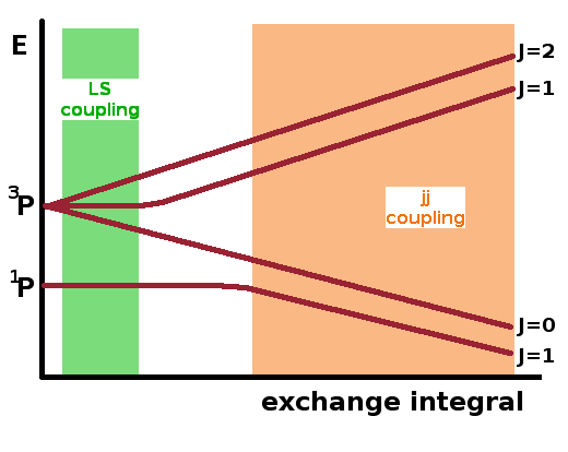
In jj coupling, the orbital angular momentum, $l$, and spin, $s$, of each electron are first coupled to form a total angular momentum, $j$, for that electron. These single-electron total angular momenta are then combined into a total angular momentum, $J$, for the group of electrons (blue calculation pathway shown in matrix above). This is in contrast to LS coupling (red pathway), where the total orbital angular momentum, $L$, and total spin, $S$, of the system are calculated first and then combined to the total angular momentum, $J$, of the whole system.
Notation: lower case for momenta of individual electrons, upper case for combined momenta.
| $j_1$→ $j_2$↴ | $\frac{1}{2}$ |
|---|---|
| $\frac{1}{2}$ | $\bbox[lightblue]{J=}|j_1-j_2|\cdots j_1+j_2\bbox[lightblue]{=0 \textrm{ or } 1}$ |
| $\frac{3}{2}$ | $\bbox[lightblue]{J=}|j_1-j_2|\cdots j_1+j_2\bbox[lightblue]{=1 \textrm{ or } 2}$ |
In general, the results from both coupling schemes are different. For example, for the 1s 2p configuration shown at the top of the page, jj coupling results in two doublets rather than a singlet and a triplet: For the 1s electron $j_1=|l_1-s_1|=l_1+s_1=\frac{1}{2}$ and for the 2p electron $j_2=|l_2-s_2|\cdots l_2+s_2=\frac{1}{2} \textrm{or} \frac{3}{2}$. These combine as shown in the table, resulting in two doublets.
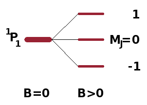
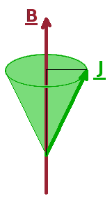
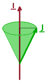
The degenerate states of a sub-shell of hydrogen, distinguished by their magnetic orbital angular momentum quantum number, $m_l$, split into energetically distinct levels when placed in a magnetic field according to their orientation relative to the field. In the same way, spin-orbit terms split according to their magnetic total angular momentum quantum number, $M_J$, into $2J+1$ separate states. This removal of degeneracy due to interaction with a magnetic field is known as the Zeeman effect and is mediated by the magnetic moment of the atom. The magnetic moment $\vec{\mu}$ is linked to the angular momentum (both orbital and spin) via the Bohr magneton, $\mu_B$, the "quantum of magnetisation": $$\vec{\mu}=-\mu_B\vec{L}-g_e\mu_B\vec{S}\qquad,$$ where $g_e$ is the electron spin g-factor, a fundamental constant very close to the value 2. Since this formula adds the electron's two angular momenta together, the magnetic moment depends on the combined angular momentum, $\vec{J}$, and the Hamiltonian for the Zeeman effect is proportional to the scalar product of the total angular momentum and the external field, i.e. the projection of one of the vectors on the other (see diagram on the left): $$\hat{H}_{\textrm{Zeeman}}\propto\vec{J}\cdot\vec{B}\qquad.$$ Each level within a term, even a singlet, therefore splits into its $2J+1$ levels with different $M_J$ quantum number. As an example, the situation for a $\mathrm{^1P_1}$ singlet is shown on the right.
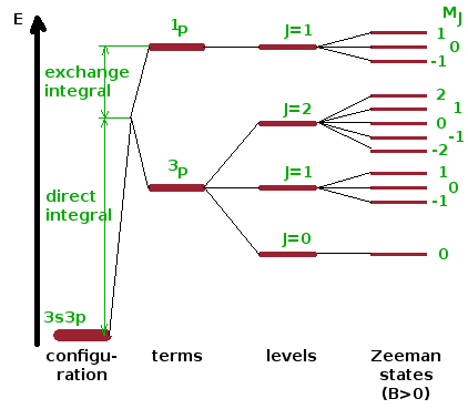
The schematic summarises the splittings due to the spin-orbit interaction: The electron configuration describes electrons in a combination of sub-shells, in the example shown a two-electron system with 3s 3p configuration. Spin-orbit coupling (in this case following the LS coupling scheme) results in a shift and a splitting into two terms due to the direct and exchange integrals, respectively. One of the term is a singlet, the other a triplet with three associated levels according to their combined total angular momentum quantum number, $J$. If placed inside a magnetic field, the Zeeman effect is observed, and each level splits into $2J+1$ Zeeman states - the extent of this splitting depends linearly on the magnitude of the magnetic field. Note that the Zeeman states are not created by the magnetic field - they are distinct states even at $B=0$, but since they are degenerate in the absence of a field, they cannot be distinguished by spectroscopic means. The diagram is not to scale - the strength of the exchange interaction is of the order of 1eV, the fine-structure levels are of the order of 10-5eV apart (GHz range), and the Zeeman splitting is of the order of 10-10eV (kHz range).
There is a further splitting below the spin-orbit related spectral detail, aptly called hyperfine interaction. It is due to the interaction between the nuclear spin, $\vec{I}$, and the combined total angular momentum, $\vec{J}$, and effectively adds another angular momentum to the vector model. Nuclear spins are the combined spins of all the protons and neutrons in the nucleus and vary between isotopes of the same element. Since nuclei are much heavier than electrons, their spin is much smaller in magnitude than that of an electron, and the nuclear spin quantum number can be zero, integer or half-integer.
The magnetic moment associated with the nuclear spin, $\vec{\mu}_I$, aligns in the magnetic field, $\vec{B}_{el}$, induced by the moving electrons. As a result, the nuclear spin plays the same role in the hyperfine interaction as the magnetic field does in the Zeeman effect: The perturbation Hamiltonian is again proportional to the scalar product of the two vectors: $$\hat{H}_{\textrm{hfs}}=-\vec{\mu}_I\vec{B}_{el}\propto\vec{I}\cdot\vec{J}\qquad.$$ The hyperfine interaction is of a strength comparable to that of the Zeeman effect at very low magnetic fields. Its states are distinguished by the quantum number $F$, which is derived from the possible orientations of $\vec{J}$ relative to $\vec{I}$ using the vector model of angular momentum in the same way as $J$ arises from the relative orientation of $\vec{L}$ and $\vec{S}$. Naturally, an atom with a nuclear spin of zero does not show any hyperfine structure splitting, and the hyperfine interaction is strongest for s-electrons due to their non-zero probability density inside the nucleus - this is known as the Fermi contact interaction.
That concludes this overview of atomic physics. We have used the Schrödinger equation to calculate the states of the hydrogen atom and their energies. Using perturbation theory in order of diminishing severity, we have added layers of complexity to the structure of the atom. As a result, a series of splittings of previously degenerate energy levels arises. We have used the vector model of angular momentum to understand how spin and orbital angular momentum couple and how the structure of complex atoms is affected by this. We have encountered spectroscopy as a means to measure the electronic structure of an atom by observing absorption and emission events between different states.