Atomic Physics

In order to adapt the solutions of the Schrödinger equation of the hydrogen-like atom to helium with its two electrons, we have added the Hamiltonians for each individual atom and added a term representing the Coulomb repulsion of the two electrons. In principle, it is straightforward to extend this approach to larger atoms with more electrons: $$\hat{H}=\sum_{i=1}^N\left(-\frac{\hbar^2}{2m}\hat{\nabla}_i^2-\frac{Ze^2}{4\pi\varepsilon_0r_i}+\sum_{j\gt i}^{N}\frac{e^2}{4\pi\varepsilon_0r_{ij}}\right)$$ The outer sum counts all the electrons, for each there is a kinetic term and a Coulomb term representing the attraction to the nucleus. The inner sum takes care of the repulsion between each pair of electrons. Since we need to count each pair only once, the inner sum starts counting at the number $i$ of the electron whose term is currently under consideration in the outer sum, hence $j\gt i$ as its lower limit.

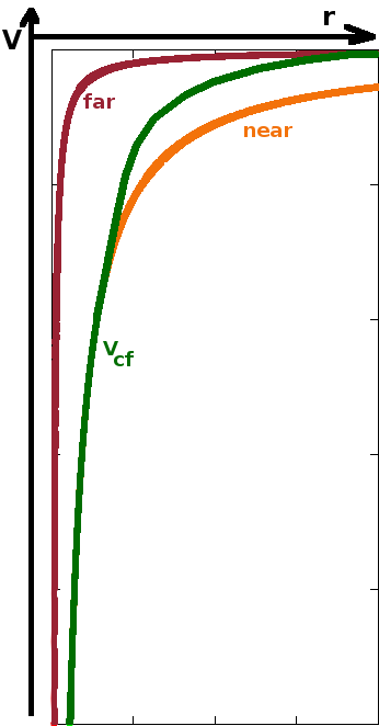
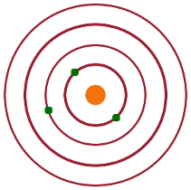
This is based on the idea that inner electrons shield part of the nuclear charge from outer electrons, effectively reducing the nuclear charge experienced by those outer electrons. The further away from the nucleus, the more electrons contribute to this shielding effect. Consider the electric field near the nucleus and far away from it: Near the nucleus, the nuclear charge is fully exposed, i.e. $$\vec{E}(\vec{r})=\frac{Ze}{4\pi\varepsilon_0r^2}\frac{\vec{r}}{r}\quad.$$ On the other extreme, far away from the nucleus, all but the outermost electron shield the nuclear charge, so only a single positive charge remains of the nuclear charge: $$\vec{E}(\vec{r})=\frac{e}{4\pi\varepsilon_0r^2}\frac{\vec{r}}{r}\quad.$$ For intermediate distances, the effective nuclear charge, $Z_{\text{eff}}(r)$, of the atom core (i.e the nucleus and all electrons up to $r$) is interpolated. It is a monotonous function of $r$, starting at the actual nuclear charge $Z$, with a significant drop at mid ranges and a long tail. $$\vec{E}_{\text{cf}}(\vec{r})=\frac{Z_{\text{eff}}\,e}{4\pi\varepsilon_0r^2}\frac{\vec{r}}{r}\quad.$$ The central field potential at a distance $r$ is the integral of the electric field from infinity inward to $r$, multiplied by the charge of an electron to interact with the field: $$V_{\text{cf}}(r)=e\int_{+\infty}^r\left|\vec{E}_{\text{cf}}(r')\right|{\rm d}r'\quad.$$

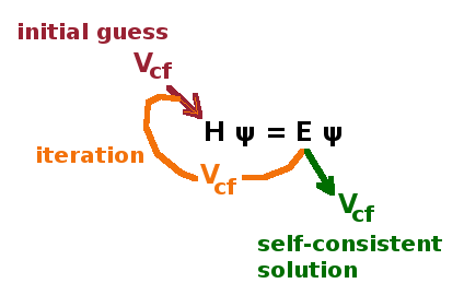
Of course the central field approximation requires that the dependence of $V_{\text{cf}}$ on the distance from the nucleus is known. As this describes the shielding of the nucleus by the inner electrons, the states of the inner electrons would have to be known in some detail in order to establish that dependence - but if we knew them, we wouldn't need to solve Schrödinger's equation... This clearly calls for a recursive numerical approach: Start by guessing a trial potential, calculate the resulting states and energy eigenvalues, refine $V_{\text{cf}}$ accordingly and re-calculate. This loop is repeated until the changes of $V_{\text{cf}}$ from one calculation to the next are acceptably small, i.e. a self-consistent solution is found. If the initial guess potential is a long way off, it will take more iterations, but the solution will usually be independent of the starting potential. Recursive numerical approaches like this are called self-consistent field techniques. Of course the wave functions change during the iteration process as well as the energy eigenvalues.

When discussing excited states of helium, we have seen that the we need to ensure that all states are anti-symmetric because of the Pauli principle. This is achieved by considering the symmetry of the space and spin functions for each state and combining them in such a way that the product is always anti-symmetric. For elements further down the periodic table, there are more electrons to be considered. Wave functions depending on all quantum numbers of all electrons are created by linear combination of the individual space and spin functions. All possible permutations of electrons (1, 2, 3...) across these wave functions ($\psi_a$, $\psi_b$, $\psi_c$...) are listed in a matrix, and the determinant of the matrix, the Slater determinant, is used as the wave function for the self-consistent field calculation. Since the sign of a determinant changes when two rows are exchanged, this ensures that the wave function is anti-symmetric. Using a Slater determinant in self-consistent field calculations is known as the Hartree-Fock technique and is one of the most common techniques of calculating multi-electron wave functions and energy levels (of atoms, molecules or crystals) from first principles.

In principle, the Hartree-Fock technique enables us to calculate all the states and their energies for any atom in the periodic table. However, the computational effort required increases rapidly with the number of electrons since the size of the Slater determinant scales with the square of the number of single-electron states involved. Given that complete occupied shells have a spherically symmetric probability density, they shield the nuclear charge very effectively. Therefore, all the alkali metals (first column of the periodic table), whose ground state has only complete shells plus a single valence electron on the outermost occupied shell, can effectively be treated in the same way as hydrogen itself, accounting for the different reduced mass of the system.

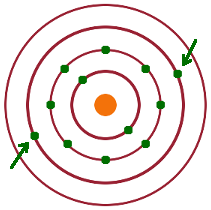
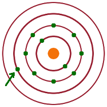
The central field approximation takes care of the effect of the inner-shell electrons. It does not, however, deal with the Coulomb repulsion between several valence electrons in the same outer shell, e.g. the two 3s electrons in magnesium (pictured). Therefore, we can apply the central field perturbation first and then extend it to cater for the interaction between the multiple valence electrons.

As seen above, the central field potential $V_{\textrm{cf}}$ contains the Coulomb interactions of each electron with the nucleus and a function $S(r)$ which represents the repulsion terms between the electrons. This assumes that $S(r)$ depends only on the distance from the nucleus but not the two angles $\theta$ and $\phi$. That is reasonable as long as there is only one valence electron. If there is one (or several) other valence electrons, their presence will shape the probability cloud for each valence state, and we need to correct for that:

$$\hat{H}=\sum_{n=1}^N\left(-\frac{\hbar^2}{2m}\hat{\nabla}_i^2\underbrace{-\frac{Ze^2}{4\pi\varepsilon_0r}+\color{red}{\cancel{\color{black}{S(r_i)}}}}_{V_{\textrm{cf}}}+\sum_{j\gt i}^N\frac{e^2}{4\pi\epsilon_0r_{ij}}-\color{red}{\cancel{\color{black}{S(r_i)}}}\right)\qquad,$$

in other words, we effectively take the radial-only function $S(r)$ out of the central-field potential again and substitute it with the full set of Coulomb repulsions. The advantage of that is that we can build on the result of the central-field perturbation by splitting the Hamiltonian into $$\hat{H}=\hat{H}_{\textrm{cf}}+\hat{H}_{\textrm{re}}\qquad,$$ where $\hat{H}_{\textrm{re}}$ is the Hamiltonian for the residual electrostatic interaction: $$\hat{H}_{\textrm{re}}=\sum_{n=1}^N\left(\sum_{j\gt i}^N\frac{e^2}{4\pi\epsilon_0r_{ij}}-S(r_i)\right)\qquad.$$ Therefore, the residual electrostatic Hamiltonian is a perturbation of the alkali (central-field) states found above, and it allows us to extend the central-field approach to the rest of the periodic table.

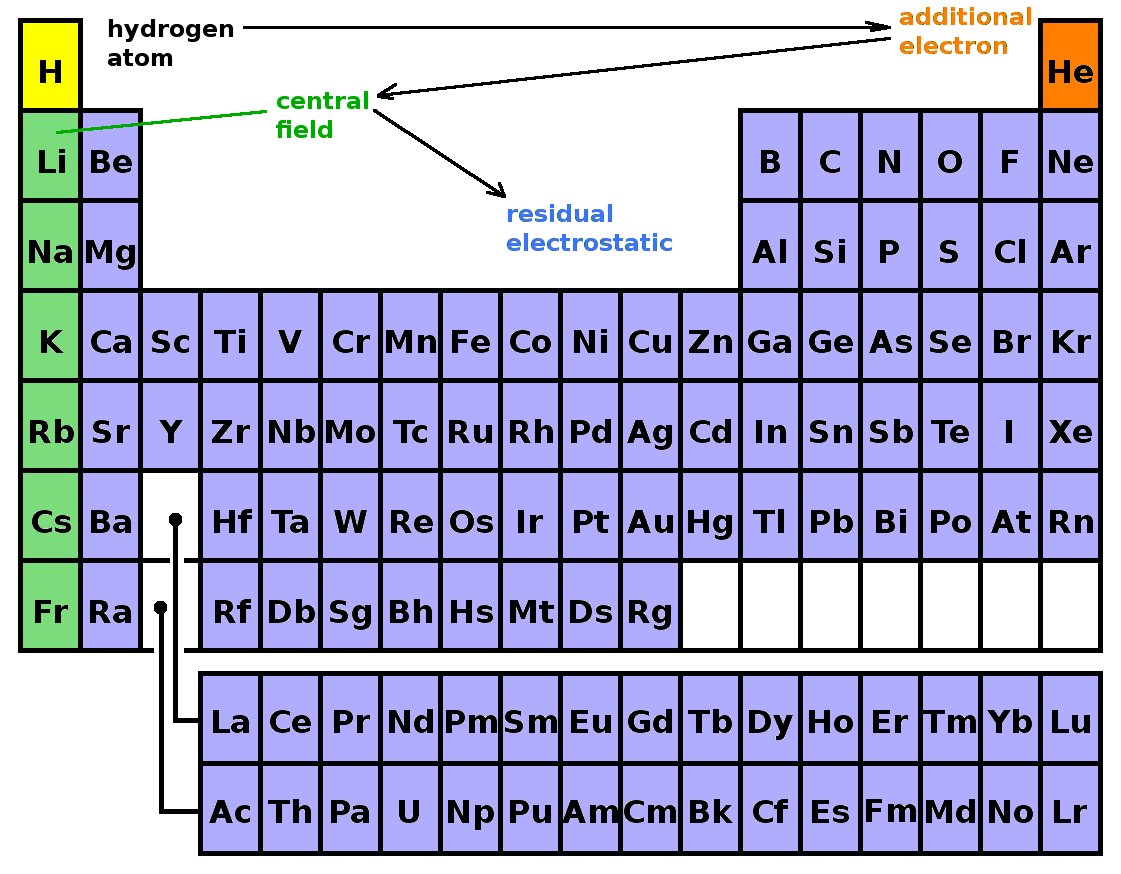
The previous sections have outlined the procedure to build up the whole periodic table by gradually adding more complexity to the wave functions of the atom. The mechanism by which this is achieved is perturbation theory: each level of complexity is introduced in terms of a perturbation Hamiltonian. The perturbation Hamiltonian is applied to the known wave functions of the unperturbed system, and corrections to the energy eigenvalues and the wave functions are calculated from that. Following that, we have a new known system, to which we can apply the next perturbation. This way, we can boot-strap the whole periodic table from the initial treatment of the Schrödinger equation of the hydrogen atom. Since perturbation theory stipulates that the perturbation must be small in comparison to the energy of the unperturbed system, the perturbations have to be applied in order of decreasing severity. In terms of building up the periodic table, the effect on the hydrogen atom of another electron is applied first, giving rise to the states of helium. Subsequently, the effect of complete filled electron shells is considered in the central-field approximation, revealing the states of the alkali metals in the first column of the periodic table. Finally, the residual electrostatic interaction takes care of additional valence electrons and thus the rest of the periodic table.

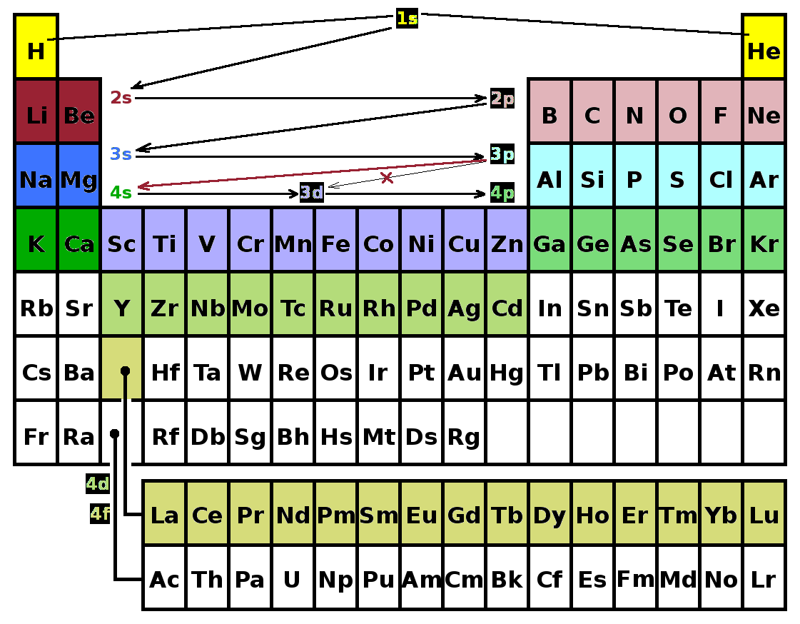
It is important to remember that perturbation theory is a technique based on approximation: each time another layer of perturbation is applied, the wave functions and energy eigenvalues are expanded into a Taylor series, and only the first-order terms (or at most a few orders) are considered. Each perturbation also results in energy shifts and splittings, e.g. states which are degenerate in hydrogen have distinct energies in helium because of the repulsion between the two electrons. As a result, the different sub-shells are populated in a definite order as the ground states of the elements in the periodic table are considered by adding more electrons. After filling the 1s subshell (helium) with two electrons with opposite spin function, the 2s subshell has lower energy than the 2p subshell due to the repulsion of the electrons. The next two elements, lithium and beryllium, therefore complete the 2s subshell, while the next six elements to neon fill the 2p subshell - three states with different $m$ quantum number for a 'p'-state ($l=1$) times two opposite spin functions for each of them. The same occurs in the third period: 3s first (up to magnesium), then 3p (up to argon). Then there is an irregularity: The 4s sub-shell (potassium and calcium) has a lower energy than the 3d sub-shell (five different orientations of the space function at $l=2$ times two spin orientations, so ten elements: scandium to zinc). Clearly, this contradicts the expectation from the original Schrödinger solution of the hydrogen atom that energy increases with $n$ quantum number - the accumulated perturbations take over and raise the energy of the 3d states above that of the 4s level. From here, the sequence continues 4p-5s-4d-5p-6s all the way down to barium. The 4f sub-shell with the lanthanides (typically shown as a separate row at the bottom of the periodic table) comes after 6s, so the cumulative effect of the perturbations results in skipping two shells at this point.

In fact, the 4f and 5d sub-shells have practically the same energy and the precise ground-state occupancies depend on exactly how many electrons beyond 6s are present. The configuration for lanthanum is $5d^1$, for cerium $4f^1\,5d^1$, but then all the electrons go into the 4f shell for praseodymium ($4f^3$) etc.

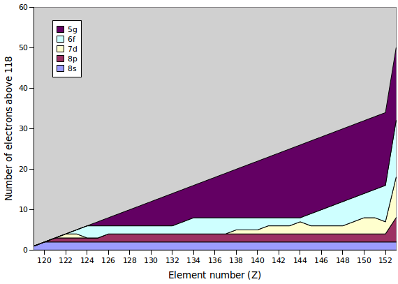
Because of these irregularities, it is not entirely clear how exactly the periodic table extends as atoms of new elements are found in accelerator experiments. Quantum-mechanical calculations suggest that the 5g, 6f, 7d and 8s sub-shells all have very similar energies when all perturbations are taken into account properly. The figure shows the predictions from an early paper (B Fricke et al., Theor Chim Acta 21 (1971) 235), but there are other studies suggesting a slightly different order of ground-state configurations. The configuration of the noble gas of the 8th period, where all sub-shells are filled, is shown on the right.