
To fill the Schrödinger equation, $\hat{H}\psi=E\psi$, with a bit of life, we need to add the specifics for the system of interest, here the hydrogen-like atom. A hydrogen-like atom is an atom consisting of a nucleus and just one electron; the nucleus can be bigger than just a single proton, though. H atoms, He+ ions, Li2+ ions etc. are hydrogen-like atoms in this context. We'll see later how we can use the exact solution for the hydrogen-like atom as an approximation for multi-electron atoms.
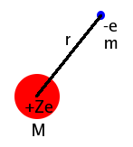
The potential, $V$ between two charges is best described by a Coulomb term, $$V(r)=-\frac{Ze^2}{4\pi\epsilon_0r}\qquad,$$ where $Ze$ is the charge of the nucleus (Z=1 being the hydrogen case, Z=2 helium, etc.), the other $e$ is the charge of the single electron, $\epsilon_0$ is the permittivity of vacuum (no relative permittivity is needed as the space inside the atom is "empty").
With the system consisting of two masses, we can define the reduced mass, i.e. the equivalent mass a point located at the centre of gravity of the system would have: $\mu=\frac{mM}{m+M}$, where $M$ is the mass of the nucleus and $m$ the mass of the electron.
Thus, the hydrogen atom's Hamiltonian is $$\hat{H}=-\frac{\hbar^2}{2\mu}\nabla^2-\frac{Ze^2}{4\pi\epsilon_0r}\qquad.$$
The Schrödinger equation of the hydrogen atom in polar coordinates is:
Both LHS and RHS contain a term linear in $\psi$, so combine:
Using the Separation of Variables idea, we assume a product solution of a radial and an angular function: $$\psi(r,\theta,\phi)=R(r)\cdot Y(\theta,\phi)\qquad.$$ Since $Y$ does not depend on $r$, we can move it in front of the radial derivative: $$\frac{\partial\psi}{\partial r}=\frac{\partial}{\partial r}RY=Y\frac{{\rm d}R}{{\rm d}r}\qquad,$$ and, similarly, $R$ does not depend on the angular variables. Thus replace $\psi$ and the differentials:
Multiply by $r^2$ and divide by $RY$ to separate the radial and angular terms:
The first and fourth terms depend on $r$ only, the middle terms depend on the angles only. They can only balance each other for all points in space if the radial and angular terms are the same constant but with opposite sign.
Therefore, we can separate into a radial equation:
and an angular equation:
where $A$ is the separation constant.
The angular part still contains terms depending on both $\theta$ and $\phi$. Another separation of variables is needed.
We'll replace $Y$ by a product of single-variable functions: $$Y(\theta,\phi)=\Theta(\theta)\cdot\Phi(\phi)\qquad.$$ Replacing $Y$ and the differentials, we have
Isolate variables in separate terms:
With $B$ as separation constant, we have a polar part: $$\bbox[lightgreen]{\frac{\sin\theta}{\Theta}\frac{\rm d}{{\rm d}\theta}\left(\sin\theta\frac{{\rm d}\Theta}{{\rm d}\theta}\right)+A\sin^2\theta}-B=0$$ and an azimuth part: $$\bbox[yellow]{\frac{1}{\Phi}\frac{{\rm d}^2\Phi}{{\rm d}\phi^2}}+B=0\qquad.$$
The azimuth equation: $$\frac{{\rm d}^2\Phi}{{\rm d}\phi^2}+B\Phi=0$$ is a 2nd order ODE with constant coefficients solved by: $$\Phi(\phi)=c_1{\rm e}^{{\rm i}m\phi}+c_2{\rm e}^{-{\rm i}m\phi}\qquad,$$ where $B=m^2$.
The angle $\phi$ is the azimuth, i.e. if you think of the atom as a globe, then $\phi$ is the longitude of the position of the electron. As long as there is no external reason to do otherwise, we can choose the "Greenwich meridian" of the atom in a mathematically convenient way by setting $c_2=0$.
Note that $m$ must be an integer number - otherwise the value of the azimuth wave function would be different for $\phi=0^{\rm o}$ and $\phi=360^{\rm o}$. In quantum terminology, $m$ is called a quantum number as it restricts the possible values of the wave function (and hence of observables) to integer multiples (quanta) of a base unit.
Thus, the azimuth part of the wave function is $\Phi_m(\phi)=c_1{\rm e}^{{\rm i}m\phi}$.
With $B=m^2$, the polar equation is: $$\frac{\sin\theta}{\Theta}\frac{\rm d}{{\rm d}\theta}\left(\sin\theta\frac{{\rm d}\Theta}{{\rm d}\theta}\right)+A\sin^2\theta-m^2=0\qquad.$$ Rearrange:
We can express the wave function as depending on $\cos\theta$ rather than on $\theta$ itself.
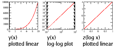
To figure this out, think of the function $y(x)=x^4$. If you plot the function logarithmically, you are effectively plotting a new function $z(\log x)=4(\log x)$ on a linear scale, where $(\log x)$ is the independent variable. Try it yourself!
Substituting $P(\cos\theta):=\Theta(\theta)$ and $x:=\cos\theta$ and hence the differential, $$\frac{\rm d}{{\rm d}\theta}=\frac{{\rm d}x}{{\rm d}\theta}\frac{\rm d}{{\rm d}x}=-\sin\theta\frac{\rm d}{{\rm d}x}\qquad,$$ leaves us with
Tidy up: $$\frac{\rm d}{{\rm d}x}\left(\sin^2\theta\frac{{\rm d}P}{{\rm d}x}\right)+\left(A-\frac{m^2}{\sin^2\theta}\right)P=0\qquad.$$ Because of $\sin^2\theta+\cos^2\theta=1$, we can further substitute $\sin^2\theta=1-\cos^2\theta=1-x^2$ and get
Apply the product rule to the first term:
Unfortunately, the coefficients in this ODE are not constant but depend on $x$, so the recipe for ODE with constant coefficients doesn't really help here. However, it is a known type of differential equation (called associated Legendre-type DE), for which a solution is known in the maths literature. The solutions are known as associated Legendre polynomials, and they contain a power series with recursive coefficients.
This means that there are two power series (for the even and odd terms, respectively) and that the coefficients of the higher terms can be calculated recursively if the first coefficient of each series, $a_0$ and $a_1$, is known. In the recursion formula, $A$ and $m$ are the constants we have from the previous parts of the solution strategy, while $n$ is the index variable of the two power series.
A series solution is only helpful if the series converges so that it can be truncated as soon as the solution is sufficiently accurate. For the recursion formula above, the series converges if $A=l(l+1)$ where $l$ is an integer number. The root coefficients of the two series, $a_0$ and $a_1$, are chosen depending on the particular value of $l$ to ensure only the convergent series survives. The first few Legendre functions are:
| $l=0$ | $l=1$ | $l=2$ | |
|---|---|---|---|
| $m=0$ | $P_0^0(x)=1$ | $P_1^0(x)=x$ | $P_2^0(x)=\frac{1}{2}(3x^2-1)$ |
| $m=1$ | --- | $P_1^1(x)=\sqrt{1-x^2}$ | $P_2^1(x)=3x\sqrt{1-x^2}$ |
| $m=2$ | --- | --- | $P_2^2(x)=3-3x^2$ |
The value of $l$ limits the choices of $m$; $m$ must have a value between $-l$ and $l$. As far as the polar part is concerned, the $\pm m$ solutions are equivalent, but the sign of $m$ makes a difference to the azimuth part as seen above.
Remember to resubstitute $P$ and $x$ when using these polar wave functions.
In the radial equation,
apply the product rule to the first term:
and divide by $r^2$:
We can't solve this straight away, but for very large $r$, the highlighted terms are forced to zero because they go reciprocal with $r$.
That leaves us with an asymptotic equation: $$\frac{{\rm d}^2R_{\infty}}{{\rm d}r^2}+\frac{2\mu E}{\hbar^2}R_{\infty}=0\qquad,$$ which is another ODE with constant coefficients. Solution:
It makes sense to use as the zero point of potential energy the energy of a free electron, i.e. in this asymptotic case, $E\to 0$ for an electron far away from the nucleus, as it is practically free. Since the presence of the positive charge in the nucleus stabilises the atom, we must look for solutions where $E$ becomes negative as the electron comes closer to the nucleus. These two conditions are met if we choose $c_4=0$ and use the fact that $E\lt 0$ to get rid of the imaginary unit.
The asymptotic solution is then $$R_{\infty}=c_3\exp{-\left(\sqrt{-\frac{2\mu E}{\hbar^2}}r\right)}\qquad.$$ The detail nearer the nucleus is expanded in a power series: $$R=R_{\infty}\sum_{q=0}^{\infty}b_qr^q\qquad.$$
This results in a series of powers of $r$ whose coefficients must all be zero to match the RHS of the differential equation. From that, a recursion formula is derived for the $b_q$, and the requirement for the series to converge produces another quantum number, $n$.
This results in the radial solution
$$R_{n,l}(r)=R_{\infty}(r)b_0\exp{\left(\frac{\mu Ze^2r}{2\pi\epsilon_0\hbar^2n}\right)}\qquad,$$
where the coefficient $b_0$ contains the $l$-dependence.
At the same time, the solution of the radial part also fixes the possible energy levels by linking them
to the quantum number $n$. The energy levels of the hydrogen-like atom are given by
The full solution of the Schrödinger equation of the hydrogen-like atom is, according to the separation approach taken:
where N is obtained by normalisation and includes the coefficients of each partial solution.
In solving the Schrödinger equation of the hydrogen atom, we have encountered three quantum numbers. Two of them, $m$ and $l$, arise from the separation constants of the $R$/$Y$ and $\theta$/$\phi$ separations. The possible values of the separation constant are restricted to integer numbers by boundary conditions (the need for the azimuth wave function to return to its value after a full 360o turn of $\phi$ and the need for the power series in the Legendre polynomial to converge to produce a physically sensible solution). The third quantum number, $n$, arises, again, from the need to have a convergent series representing the non-asymptotic part of the radial function.
| $n$= | 1 | 2 | 3 | ... | |||||||||||
| $l$= | 0 | 0 | 1 | 0 | 1 | 2 | 0...(n-1) | ||||||||
| $m$= | 0 | 0 | -1 | 0 | +1 | 0 | -1 | 0 | +1 | -2 | -1 | 0 | +1 | +2 | -l...+l |
The quantum numbers are not independent; the choice of $n$ limits the choice of $l$, which in turn limits the choice of $m$. A fourth quantum number, $s$, does not follow directly from solving the Schrödinger equation but is to do with spin. The possible combinations of quantum numbers are given in the table.
Note that the energy of a state (i.e. of a wave function) depends only on $n$ but not on the other quantum numbers. This degeneracy is only strictly true for the hydrogen-like atom; any approximate solutions for higher atoms cause a dependence of the energy eigenvalue of a state on all quantum numbers.
All of the above mean the same thing: a solution of the Schrödinger equation. The term state is often used when dealing with spectroscopic transitions, e.g. when an electron is excited from a state with a lower energy into one with a higher energy, i.e. it changes from a wave function with a smaller to one with a higher value of n. The term orbital (a word coined in reference to the distinct electron orbits of Bohr's model of the atom on which electrons were supposed to move without radiating) stresses the interpretation of the wave function in terms of the probability of locating an electron. This often occurs in the context of chemical bonds.
Knowing the energy eigenvalues and eigenfunctions of hydrogen, we can now determine the spectrum of hydrogen (and the sun) and the shapes of the electron probability clouds of the various states.