
The energy of a state with quantum number $n$ is $$E_n=-\frac{\mu Z^2e^4}{8\epsilon_0^2h^2n^2}\qquad.$$ For transitions between two states, the energy difference between the two states must either be supplied (excitation) or emitted. Since the states have discrete energy levels, only fitting energy quanta can be involved in the transition. The energy difference between two adjacent states is $$\Delta E_{n_1,n_2}=-\frac{\mu Z^2e^4}{8\epsilon_0^2h^2}\left(\frac{1}{n_1^2}-\frac{1}{n_2^2}\right)\qquad;$$ thus spectral lines occur only at the corresponding energies (frequencies, wavelengths, wavenumbers,...).
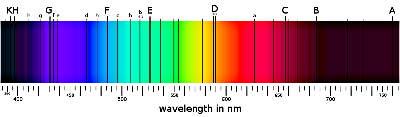
This had been observed long before quantum mechanics - the first observations concern the Sun's spectrum. The constants in front of the bracket are collectively known as the Rydberg constant, $R_H$; its value was determined experimentally before quantum physics provided the link to the fundamental constants.
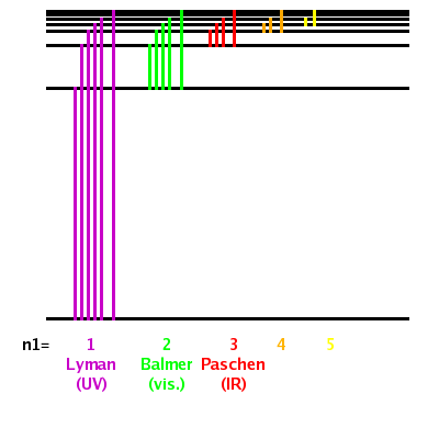
The different series of spectral lines discovered by Lyman, Balmer, and Paschen, correspond to the excitations from the $n$=1,2,3 states.
The wave function itself, a complex function with positive and negative values, doesn't tell us much about the structure of the atom or any connectivity it may have with other atoms. The complex square of the wave function represents the probability density of finding the electron at a given point in space when one looks (i.e. does an experiment). It does not say anything about where the electron actually is at any moment, the solutions of the Schrödinger equation only refer to which states are observable. The act of measuring throws the system into one of the eigenstates that are solutions of the Schrödinger equation.
A recurrent idea of statistics is that temporal averages are equivalent to ensemble averages, i.e. look for a while at one object moving randomly and you will see the same set of orientations that you would see when taking a snapshot of many identical objects moving randomly. In the same way, we can interpret the probability density as a representation of the electron density in an atom, molecule, or solid.
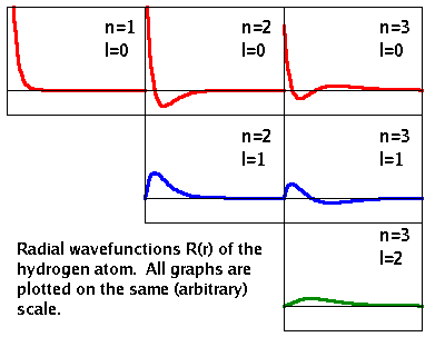
The radial solutions of the Schrödinger equation of the hydrogen atom, $R(r)$, are plotted on the right. Each time the quantum number $n$ increases, an additional node is created. At $n$=1, the radial function is all positive. Its maximum is at $r$=0, i.e. the point in space with the highest probability density of finding the electron is actually inside the nucleus! That is why the term probability density is used: As we move outward along the radius, the volume of a shell of equal thickness is getting larger and larger, thereby spreading out the probability over a larger volume.
Each time the quantum number $l$ is increased, one of the spherical nodes disappears again. It is replaced by a planar node that goes through the nucleus. Therefore, only $l$=0 electrons have a finite probability density at the nucleus.
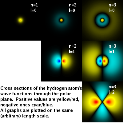
The diagram on the right shows cross sections of the full wave function $\psi(r,\vartheta,\varphi)$ in the polar ($r$-$\vartheta$) plane. This representation highlights the transformation of spherical nodes into planar nodes as $l$ increases.
It is also apparent that the wave function is spreading out into space as $n$ increases, i.e. that electrons with a small $n$ are, on balance, nearer the nucleus. Given that the energy eigenvalue increases with $n$, that matches the semi-classical expectation that electrons have a lower energy if they are deep down in the Coulomb potential.
One more observation: As $l$ increases, the additional planar nodes cause the wave function to become less and less symmetric. This is compensated by the increasing number of equivalent states having the same $n$ and $l$ but different $m$. (In the diagram, only $m$=0 states are shown.) All (2$l$+1) states with the same value of $n$ and $l$ together form a perfectly spherical distribution of probability density.
Note that since the probability density is the square of the wave function, it makes no difference if the wave function is positive or negative.
| l= | 0 | 1 | 2 | 3 | 4... |
| letter: | s | p | d | f | g (then continue alphabetically) |
Instead of describing a state by listing the values of its quantum numbers, a common practice is to refer to them by main quantum number, $n$, followed by a letter representing the value of $l$ as shown in the table.
Thus, a 2p state is one with $n$=2 and $l$=1 (the $m$=-1,0,+1 cases are sometimes distinguished as 2px, 2py, and 2pz); a 3d state is one with $n$=3 and $l$=2.
We now have accurate wave functions and their energies for hydrogen-like atoms. Solving the Schrödinger equation analytically is impossible for more complex systems. Instead, we can use the known system as a base and add complexity gradually, adjusting the wave functions and energies step by step. This perturbation approach also allows us to calculate the effect of interactions with the electron system, such as the interaction of radiation with matter on which spectroscopy is based.