
| Boltzmann | |||||
| Bose-Einstein | |||||
| Fermi-Dirac | |||||
Classical Boltzmann statistics assumes that the system is made up of
distinguishable particles.
In the dice metaphor this corresponds to using coloured dice to ensure we can distinguish
![]()
![]() from
from
![]()
![]() .
In general, this is appropriate in a classical system because we can, in principle
(although with difficulty in practice), measure the position and trajectory of each
particle and, by keeping track of them, distinguish them from one another.
.
In general, this is appropriate in a classical system because we can, in principle
(although with difficulty in practice), measure the position and trajectory of each
particle and, by keeping track of them, distinguish them from one another.
The situation
is different in quantum mechanics because of
Heisenberg's uncertainty principle,
which puts a fundamental lower limit on the product of the uncertainties of position and
momentum of any measurement. Therefore, an alternative statistical approach is needed for
indistinguishable particles.
In the dice metaphor, we can achieve this by using identically coloured dice. Now there is
no difference between
![]()
![]() and
and
![]()
![]() ,
and the number of microstates contributing to each macrostate is reduced accordingly.
,
and the number of microstates contributing to each macrostate is reduced accordingly.
For certain quantum particles, an additional constraint applies: Particles with half-integer spin (e.g. electrons) obey the Pauli exclusion principle; they cannot occupy the exact same quantum state, i.e. have exactly the same set of quantum numbers. When playing dice, this is the equivalent of rejecting all those throws that result in the same number on several dice. Particles for which this applies are called fermions; they obey the Fermi-Dirac statistics. Particles with integer spin can congregate in the same state and therefore aren't subject to this constraint. They are known as bosons and are described by the Bose-Einstein statistics.
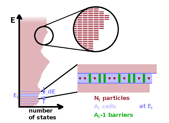
Bose-Einstein statistics describes indistinguishable, non-interacting quantum particles. The derivation of the distribution function follows the same method used when deriving the Boltzmann distribution, but the statistical weight of the macrostates is different. Consider a situation where energy levels are close together. We can treat all states within a narrow range ${\rm d}E$ of energies as essentially degenerate. If there are $A_i$ levels within the range, then we need to slice up the range into $A_i$ "cells" using $A_i-1$ barriers between them. In addition, we need to distribute the $N_i$ particles in this energy range across those cells. In effect, we have a mixed distribution of barriers and particles across the size of the degenerate energy range. The number of microstates within $[E_i,E_i+{\rm d}E]$ is then $$\frac{(N_i+A_i-1)!}{N_i!(A_i-1)!}\qquad.$$ The numerator counts all objects (barriers and particles) to be distributed, while the denominator removes the duplicates due to the fact that we can swap any two particles without making a difference, neither will swapping any two barriers create a distinguishable microstate. However, swapping a barrier and a particle will change the size of two of the cells, resulting in a different microstate that contributes to the statistical weight of the macrostate. Up to this point, this description only deals with the situation in the energy range at $E_i$, but a similar situation applies to all the other energy ranges, too. Therefore, the statistical weight of a macrostate is the product of all the individual weights of each of the energy ranges: $$\Omega=\prod_i{\frac{(N_i+A_i-1)!}{N_i!(A_i-1)!}}\approx\prod_i{\frac{(N_i+A_i)!}{N_i!(A_i)!}}\qquad.$$ If the system is large, the 1 is negligible compared to the number of particles.
The rest of the derivation follows the familiar pattern. First, take the logarithm of the statistical weight: $$\ln\Omega=\sum_i\ln(N_i+A_i)!-\sum_i\ln N_i!-\sum_i\ln A_i!\qquad.$$ Some of the sums cancel out after applying Stirling's formula: $$\qquad=\sum_i(N_i+A_i)\ln(N_i+A_i)\color{red}{\cancel{\color{black}{-\sum_i(N_i+A_i)}}}-\sum_iN_i\ln N_i\color{red}{\cancel{\color{black}{+\sum_i N_i}}}-\sum_iA_i\ln A_i\color{red}{\cancel{\color{black}{+\sum_iA_i}}}\qquad.$$ To find the most probable macrostate, we need to calculate the total differential of $\ln{\Omega}$ and set it to zero: $${\rm d}\ln\Omega=\sum_i{\frac{{\rm d}}{{\rm d}N_i}(N_i+A_i)\ln(N_i+A_i){\rm d}N_i}-\sum_i{\frac{{\rm d}}{{\rm d}N_i}N_i\ln N_i{\rm d}N_i}-\sum_i{\color{red}{\cancel{\color{black}{\frac{{\rm d}}{{\rm d}N_i}A_i\ln A_i}}}{\rm d}N_i}\qquad.$$ The final sum is zero because it contains the derivative of a constant term. The other two sums need an application of the product rule: $$\qquad=\color{red}{\cancel{\color{black}{\sum_i\frac{N_i+A_i}{N_i+A_i}{\rm d}N_i}}}+\sum_i\ln(N_i+A_i){\rm d}N_i\color{red}{\cancel{\color{black}{-\sum_i\frac{N_i}{N_i}{\rm d}N_i}}}-\sum_i\ln N_i{\rm d}N_i\qquad.$$ Now the first and third term cancel, and the other two can be combined: $$\qquad=\sum_i\ln\frac{N_i+A_i}{N_i}{\rm d}N_i=\sum_i\ln\left(\frac{A_i}{N_i}+1\right){\rm d}N_i\overset{!}{=}0\qquad.$$ At the same time, the total number of particles and the total energy of the system are maintained if we are considering (as in the derivation of the Boltzmann distribution) a closed system: $$N=\sum_iN_i\quad\Rightarrow\quad{\rm d}N=\sum_i{\rm d}N_i\overset{!}{=}0$$ $$E=\sum_iN_iE_i\quad\Rightarrow\quad{\rm d}E=\sum_iE_i{\rm d}N_i\overset{!}{=}0\qquad.$$ The three equations are combined using Lagrange multipliers: $$\sum_i\left[\ln\left(\frac{A_i}{N_i}+1\right)+a+bE_i\right]{\rm d}N_i\overset{!}{=}0\qquad,$$ leading to a population of a specific level, taking into account the extent of degeneracy: $$\frac{N_i}{A_i}=\frac{1}{\exp{\left(-a-\frac{E_i}{k_BT}\right)}-1}\qquad.$$ Apart from the degeneracy, the difference from the Boltzmann distribution lies in the -1 in the denominator.
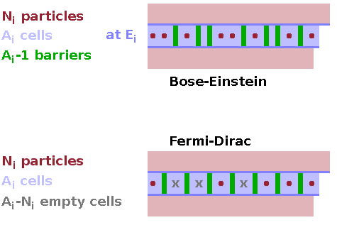
The Fermi-Dirac statistics for indistinguishable particles with half-integer spin can be derived in a very similar way. Since fermions cannot be in the exact same quantum state (energy level), all the cells in the degenerate energy range can only either be empty or occupied by a single particle. This means we don't need to distribute barriers since they are in fixed locations - each cell is the same size. The contribution of each energy range to the statistical weight is then the number of combinations of empty ($A_i-N_i$) and occupied ($N_i$) cells, divided by the number of indistinguishable combinations due to either swapping two empty cells or two occupied cells. As before, the total statistical weight is the product of these contributions from each energy range: $$\Omega=\prod_i\frac{((A_i-N_i)+N_i)!}{N_i!(A_i-N_i)!}=\prod_i\frac{A_i!}{N_i!(A_i-N_i)!}\quad.$$ Again, we take the logarithm, $$\ln\Omega=\sum_i\ln(A_i!)-\sum_i\ln(N_i!)-\sum_i\ln[(A_i-N_i)!]\qquad,$$ apply Stirling's formula, $$\qquad=\sum_iA_i\ln A_i\color{red}{\cancel{\color{black}{-\sum_iA_i}}}-\sum_iN_i\ln N_i\color{red}{\cancel{\color{black}{+\sum_iN_i}}}-\sum_i(A_i-N_i)\ln(A_i-Ni)\color{red}{\cancel{\color{black}{+\sum_i(A_i-N_i)}}}\qquad,$$ and compare with Bose-Einstein: $$\ln\Omega_{BE}=\color{red}{-}\sum_iA_i\ln A_i-\sum_iN_i\ln N_i\color{red}{+}\sum_i(A_i\color{red}{+}N_i)\ln(A_i\color{red}{+}N_i)$$ The formula is very similar; only the four highlighted signs are different for the two quantum statistics. By carrying through these sign changes, we have for the population of a particular energy range: $$\frac{N_i}{A_i}=\frac{1}{\exp{\left(-a-\frac{E_i}{k_BT}\right)}\color{red}{+}1}$$ The only difference is the +1 in the denominator.
Degeneracy, i.e. the observation that quantum-mechanically distinct states (states where at least some of the quantum numbers have different values) can have the same energy, plays a key role in the derivation of the two quantum statistics, the Bose-Einstein and the Fermi-Dirac distribution. The reason for this is that we derive the statistical weight of each macrostate by investigating a series of energy levels, each of which contains many degenerate quantum states.
To work out the role of degeneracy in the quantum distributions, we will investigate one particular quantum mechanical model, the particle in a box in this respect. We have already used this model previously to determine the translational partition function. The model is based on the idea that the wave function of a particle trapped in a box must be a standing wave pinned at the opposite sides of the box. Therefore, all the possible wave functions are harmonics of a fundamental wave where half an oscillation period ($\pi$) fits exactly into the size of the box, $a$: $$\psi_n(x)=\sin\left(\frac{n\pi x}{a}\right)\qquad.$$ The different states (wave functions) are distinguished by a quantum number, $n=1,2,3\dots$, in this case effectively the order of the harmonic of the wave. Quantum mechanics also predicts the energy eigenvalue of each of these states: $$E_n=\frac{n^2h^2}{8ma^2}\qquad,$$ i.e. the energy of the states grows with the square of the quantum number.
| $n_x$ | $n_y$ | $n_z$ | $n^2$ | |
|---|---|---|---|---|
| 1 | 1 | 1 | 3 | |
| 2 | 1 | 1 | 6 | |
| 1 | 2 | 1 | 6 | |
| 1 | 1 | 2 | 6 | |
| 2 | 2 | 1 | 9 | |
| 2 | 1 | 2 | 9 | |
| 1 | 2 | 2 | 9 | |
| 3 | 1 | 1 | 11 | |
| 1 | 3 | 1 | 11 | |
| 1 | 1 | 3 | 11 | |
| 2 | 2 | 2 | 12 | |
| 3 | 2 | 1 | 14 | |
| 3 | 1 | 2 | 14 | |
| 2 | 3 | 1 | 14 | |
| 2 | 1 | 3 | 14 | |
| 1 | 3 | 2 | 14 | |
| 1 | 2 | 3 | 14 |
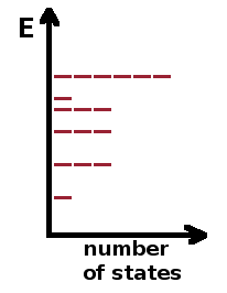
In this system, degeneracy comes about when we extend the problem from one to more dimensions. In 3D, we have a quantum number in each of the dimensions, and the total quantum number is the root mean square of the individual quantum numbers: $$n^2=n_x^2+n_y^2+n_z^2\qquad.$$ The table shows the lowest-energy states of this combined 3D system, and the Fig. is a graphical representation of the distribution of states along the energy axis. As can be seen, we will have six states with the same energy if the quantum numbers for all three directions are different, three states if two quantum numbers are equal and the other different, and only one state if the quantum numbers of all directions co-incide. As a result, the spacing of the energy levels along the energy axis also varies. This demonstrates how a system characterised by several quantum numbers will show degeneracy ($g_i$ states with the same energy, $E_i$) even if there is a single energy eigenvalue for each value of each quantum number individually.
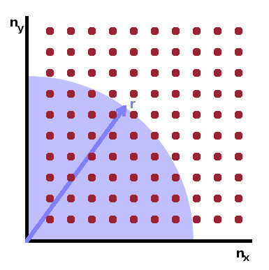
In order to count the number of states at each energy, we can draw a diagram with the quantum numbers for each spatial direction on the axes - the situation for a two-dimensional particle in a box is shown in the Fig. This gives rise to the notion of phase space, i.e. a space whose axes are not the spatial dimensions but rather the quantum numbers of the system. Since the quantum numbers distinguish different states, we can count the number of states by measuring the size of an area (in 2D) or volume (in 3D) in phase space.
The radius of a sphere in phase space is the total quantum number, $n$, the root-mean-square of the individual quantum numbers along the different axes: $$n=\sqrt{n_x^2+n_y^2+n_z^2}=\sqrt{\frac{8ma^2E}{h^2}}\qquad.$$ The number of states within a sphere of radius $n$ is $N=\frac{4}{3}\pi n^3$, but given that all quantum numbers in the particle-in-a-box model are positive, we should only count one octant of the sphere (where $n_x,n_y,n_z\gt 0$), so the number of states up to $n$ is $$N=\frac{1}{8}\cdot\frac{4}{3}\pi n^3=\frac{4\pi}{3}\left(\frac{2ma^2E}{h^2}\right)^{\frac{3}{2}}\qquad.$$
By differentiating this with respect to the energy we can derive the density of states, $$g(E)=\frac{{\rm d}N}{{\rm d}E}=\frac{4\pi}{3}\left(\frac{2ma^2}{h^2}\right)^{\frac{3}{2}}\frac{3}{2}E^{\frac{1}{2}}=\frac{2\pi a^3}{h^3}(2m)^{\frac{3}{2}}\sqrt{E}\qquad,$$ a continuous expression of the discrete concept of degeneracy - instead of referring to the number of states at a particular energy level, it gives the number of states in an infintesimally narrow energy band at a particular energy. For the particle in a 3D box, the density of states increases with the square root of the energy.
Just as we need to take into account discrete degeneracy when using Boltzmann statistics to distribute particle across discrete energy levels, we need to take into account the density of states when using the quantum statistics, which assume that states are very close together in energy. Therefore, a bundle of states at a particular energy will have a statistical weight of $$\Omega_i=\frac{g_i^{N_i}}{N_i!}\qquad.$$
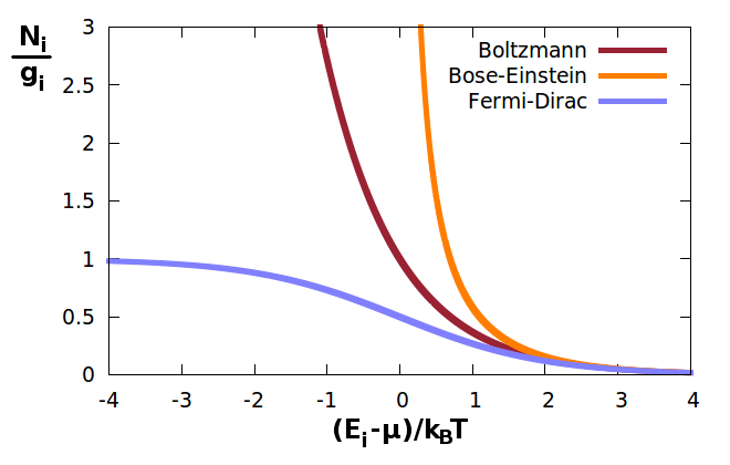
To summarise, the three particle statistics are summarised below: $$\begin{eqnarray} \textbf{Boltzmann}&:&\frac{N_i}{g_i}=\frac{1}{\exp{\left(-\frac{E_i-\mu}{k_BT}\right)}}\\ \textbf{Bose-Einstein}&:&\frac{N_i}{g_i}=\frac{1}{\exp{\left(-\frac{E_i-\mu}{k_BT}\right)}\color{red}{-}1}\\ \textbf{Fermi-Dirac}&:&\frac{N_i}{g_i}=\frac{1}{\exp{\left(-\frac{E_i-\mu}{k_BT}\right)}\color{red}{+}1} \end{eqnarray}$$ chemical potential, $\mu=ak_BT$
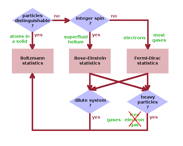
The figure provides a decision matrix to determine which statistics is appropriate along with some classes of systems where each would be applicable.
Now that we have statistics for both distinguishable and indistinguishable particles, we need to deal with the assumption made so far that the particles do not interact. This is achieved by using ensemble statistics.