
Thermodynamic systems typically contain a large number of particles. State variables describe the behaviour of a system as a whole without considering the properties of individual particles or the interactions between them. There are both practical and fundamental reasons that we cannot measure the state of a system by determining each particle's state individually and averaging (for intensive variables) or adding them all up (for extensive ones): there are too many particles, and quantum mechanics tells us that many observables cannot be measured simultaneously with precision. It is therefore appropriate to use statistics to analyse the behaviour of many-particle systems and determine their state variables.
It is useful to consider a game of dice in order to understand the use of statistics when dealing
with large systems. The average total score from any throw of any number of dice is always 3.5 times the
number of dice, but the
probability distribution
of scores changes drastically as the number of dice
thrown increases. For a single dice, all six possible values have the same probability. If two
dice are thrown, the scores range from 2 to 12, but these extreme values are less likely than the
average value of 7. The reason is that there is only one combination that realises a score of
2 but six different combinations to achieve a 7. This assumes that we can distinguish the two dice
(e.g. by their colour) and can therefore tell e.g.
![]()
![]() from
from
![]()
![]() .
The probability distribution for two dice has a triangular shape.
.
The probability distribution for two dice has a triangular shape.
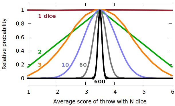
For three dice, working out the possible combinations begins to become cumbersome - never mind a mole of dice! The distribution is a binomial distribution and gets progressively narrower as the number of dice increases. The Fig. shows computer-simulated distributions for a million throws of 1, 2, 3, 10, 60 and 600 dice, normalised vertically and horizontally to the probability of the peak of the function and the average value, respectively. From about ten dice, the curve resembles very closely a Gaussian distribution, characterised by its mean, $x_0$, and standard deviation, $\sigma$: $$f(x)=\frac{1}{\sqrt{2\sigma^2\pi}}\exp{-\frac{(x-x_0)^2}{2\sigma^2}}\qquad.$$
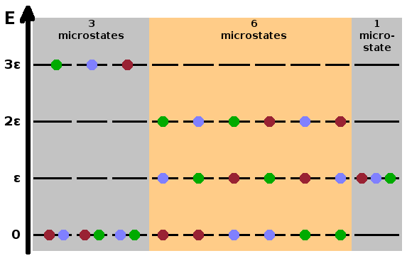
In thermodynamic terms, the dice are replaced by particles, the score each dice shows with the energy of
a particle, and the distribution of total scores with the distribution of particles over available energy levels.
We define as a
microstate
a particular distribution of a set of particles across the energy levels. In dice terms, both
![]()
![]() and
and
![]()
![]() would be different microstates of our "system" of dice. A
macrostate
on the other hand is the total score of all the dice or distribution of particles across energy
levels without consideration of which particle is in which level. The Fig. shows the ten possible
microstates of three particles distributed across four equidistant energy levels while maintaining
a constant total energy. The macrostate on the left consists of three microstates - in each case,
one of the particles is in the highest and the other two in the lowest level. The three microstates
arise from assigning the higher energy to a different particle. The second macrostate has six
contributing microstates: the energy of the highest-energy particle is dropped by one notch, and one
of the other particles is lifted up by one level, resulting in three occupied levels and therefore
six combinations. Finally, the third macrostate, where all three particles are in the second-lowest
level, has only one microstate since swapping particles in the same level makes no difference - the
equivalent of a
would be different microstates of our "system" of dice. A
macrostate
on the other hand is the total score of all the dice or distribution of particles across energy
levels without consideration of which particle is in which level. The Fig. shows the ten possible
microstates of three particles distributed across four equidistant energy levels while maintaining
a constant total energy. The macrostate on the left consists of three microstates - in each case,
one of the particles is in the highest and the other two in the lowest level. The three microstates
arise from assigning the higher energy to a different particle. The second macrostate has six
contributing microstates: the energy of the highest-energy particle is dropped by one notch, and one
of the other particles is lifted up by one level, resulting in three occupied levels and therefore
six combinations. Finally, the third macrostate, where all three particles are in the second-lowest
level, has only one microstate since swapping particles in the same level makes no difference - the
equivalent of a
![]()
![]()
![]() throw.
throw.
The underlying assumption in this concept is that all microstates individually are equally probable - a
![]()
![]() is as likely as a
is as likely as a
![]()
![]() or any other combination of the two coloured dice. The extreme situation where one particle contains the
whole energy of the system is as likely as any one of the many combinations of the particles
across the energy levels.
or any other combination of the two coloured dice. The extreme situation where one particle contains the
whole energy of the system is as likely as any one of the many combinations of the particles
across the energy levels.
Because there are more different microstates contributing to the macrostates near the peak of the probability distribution, we can define the statistical weight, $\Omega$, as the number of microstates contributing to a macrostate. For distinguishable, non-interacting particles (or coloured dice), the statistical weight is given by $$\Omega=\frac{N!}{\prod_rN_r!}\qquad.$$ The numerator counts all the permutations of the $N$ particles over the $r$ energy levels, and the denominator removes the duplicate microstates arising from the fact that we can swap even distinguishable particles without making a difference if they are in the same energy level. The product symbol, $\prod_r$, signifies a product running over all energy levels. The statistical weight of the first macrostate shown in the Fig. above is therefore $$\color{grey}{\Omega=\frac{3!}{1!\;0!\;0!\;2!}=\frac{6}{2}=3}\qquad.$$
When distributing the particles over the energy levels, we have to maintain two additional conditions: The number of particles doesn't change since we're not adding or removing material from the system - the system is a closed system: $$N=\sum_{i=0}^{r-1}N_i\qquad.$$ In a closed system, we also do not allow any flows of energy into or out of the system; it is enclosed in adiabatic walls. Therefore, the total energy, $E$, also remains constant: $$E=\sum_{i=0}^{r-1}N_i\epsilon_i\qquad.$$ As seen above, probability distributions become very narrow once numbers get large. In a macroscopic system, the probability is almost entirely concentrated in the most probable macrostate. It is therefore safe to assume that the particles of any macroscopic system will be in a distribution which corresponds to one of the many microstates constituting the most probable macrostate. Particles will change energy levels, i.e. the precise microstate of the system will change dynamically, but it is very unlikely that these dynamic processes will ever produce a population pattern that is significantly different from that representing the most probable macrostate.
In order to work out the populations of the different energy levels for the most probable macrostate, we need to find the location of the maximum of the distribution function, i.e. of the statistical weight. Since the numbers are so large, this is difficult. However, since the logarithm of a function peaks at the same place as the function itself, we might as well search for the maximum of $\ln\Omega$, which is much smaller. By taking the logarithm, the fraction turns into a difference, and the product into a sum:
$$\ln{\Omega}=\ln{\frac{N!}{\prod_{i=0}^{r-1}N_i!}}=\ln{N!}-\sum_{i=0}^{r-1}\ln{N_i!}\qquad\qquad\color{grey}{\left[\ln{(ab)}=\ln{a}+\ln{b}\right]}\qquad.$$
The Stirling formula is an approximation that enables us to lose the factorials: $$\ln{x}!\approx x\ln{x}-x$$ as long as $x$ is a large number. Applying it to the logarithm of the statistical weight, we have $$\ln{\Omega}=N\ln{N}\color{red}{\cancel{\color{black}{-N}}}-\sum_{i=0}^{r-1}N_i\ln{N_i}+\color{red}{\cancel{\color{black}{\sum_{i=0}^{r-1}N_i}}}\qquad,$$ where the second and fourth terms cancel out because the sum of the populations of all energy levels is the total number of particles.
To find the peak, we have to find the point at which the function doesn't change if we change any of the populations $N_i$ by an infinitesimal amount ${\rm d}N_i$. In other words, the total differential of $\ln{\Omega}$ must be zero. Since $N$ is a constant, the first term of $\ln{\Omega}$ doesn't change. Each term of the sum is differentiated individually with respect to 'its' population $N_i$:
$${\rm d}\ln{\Omega}=-\sum_i\frac{\partial}{\partial N_i}N_i\ln{N_i}{\rm d}N_i\qquad\qquad \color{grey}{\left[{\rm d}f(x,y)=\frac{\partial f}{\partial x}{\rm d}x+\frac{\partial f}{\partial y}{\rm d}y\right]}$$
The product rule applies, and as the second term evaluates to 1 it can be neglected compared to $\ln{N_i}$:
$$\qquad=-\sum_i\left(\frac{\partial N_i}{\partial N_i}\ln{N_i}+N_i\frac{\partial\ln{N_i}}{\partial N_i}\right){\rm d}N_i =-\sum_{i=0}^{r-1}\left(\ln{N_i}+\color{red}{\cancel{\color{black}{N_i\frac{1}{N_i}}}^{\ll}}\right){\rm d}N_i\qquad,$$
leaving $$\qquad\approx -\sum_i\ln{N_i}{\rm d}N_i\overset{!}{=}0\qquad,$$ which has to equal zero at the maximum of the distribution. At the same time, the number of particles and total energy must also be kept constant: $${\rm d}N=\sum_i{{\rm d}N_i}\overset{!}{=}0$$ $${\rm d}E=\sum_i{\epsilon_i{\rm d}N_i}\overset{!}{=}0$$ The three equations can be solved simultaneously using the method of the Lagrange multipliers. This is a method frequently used in constrained optimisation problems such as non-linear curve fitting subject to constraints. The idea is that the constraints ($N$ and $E$) are added to the main equation ($\ln{\Omega}$) with unknown coefficients (the multipliers). Here, this produces an equation for each term of the sum (i.e. each energy level): $$(-\ln{N_i}+a+b\epsilon_i){\rm d}N_i\overset{!}{=}0\qquad.$$ Ignoring the trivial case ${\rm d}N_i=0$, this requires that $$N_i={\rm e}^{a+b\epsilon_i}\qquad,$$ producing a useful link between the population $N_i$ of a level and its energy $\epsilon_i$. The total number of particles is the sum of all the population numbers: $$N=\sum_iN_i=\sum_i{\rm e}^{a+b\epsilon_i}={\rm e}^a\sum_i{\rm e}^{b\epsilon_i}\qquad,$$ where ${\rm e}^a$ is the same for all levels and can therefore be taken out of the sum. After re-arranging this for ${\rm e}^a$, $${\rm e}^a=\frac{N}{\sum_i{\rm e}^{b\epsilon_i}}\qquad,$$ we can substitute this factor in the equation for the population of an individual level: $$N_i={\rm e}^{a+b\epsilon_i}={\rm e}^a{\rm e}^{b\epsilon_i}=\frac{N{\rm e}^{b\epsilon_i}}{\sum_i{\rm e}^{b\epsilon_i}}\qquad.$$ The constant $b$ must be a reciprocal energy in order for the exponent to be dimensionless. We identify this with the thermal energy, $k_BT$. This produces the Boltzmann distribution, i.e. the distribution of particles across energy levels in thermal equilibrium:
The sum in the denominator is known as the partition function. Provided we have either a model (typically from quantum mechanics) that predicts the energy levels or experimental data (typically spectroscopic data) that determines them, we can calculate the equilibrium populations of the levels using the partition function and the Boltzmann distribution.
Once the partition function of a system is known, its state variables can be calculated without the need to deal with the individual energy levels. As an example, the internal energy, $U$, of a system can be calculated directly from the partition function. The internal energy is the sum of the energies of all energy levels of the system, weighted by their populations. The populations can be taken from the Boltzmann distribution: $$U=\sum_iN_i\epsilon_i=\frac{N\sum_i\epsilon_i\exp{\left(-\frac{\epsilon_i}{k_BT}\right)}}{\sum_i\exp{\left(-\frac{\epsilon_i}{k_BT}\right)}}\qquad.$$ By differentiating the partition function with respect to temperature, $$\frac{{\rm d}z}{{\rm d}T} =\frac{{\rm d}}{{\rm d}T}\sum_i\exp{\left(-\frac{\epsilon_i}{k_BT}\right)} =\sum_i\exp{\left(-\frac{\epsilon_i}{k_BT}\right)}\left(-\frac{\epsilon_i}{k_B}\right)\left(-\frac{1}{T^2}\right) =\sum_i\frac{\epsilon_i\exp{\left(-\frac{\epsilon_i}{k_BT}\right)}}{k_BT^2}\qquad,$$ we can see that the sum in the numerator of the internal energy is linked to $\frac{{\rm d}z}{{\rm d}T}$, while the sum in the denominator is the partition function itself: $$U=\frac{Nk_BT^2\frac{{\rm d}z}{{\rm d}T}}{z}=Nk_BT^2\frac{{\rm d}\ln{z}}{{\rm d}T} \qquad\qquad\color{grey}{\left[\frac{{\rm d}}{{\rm d}x}\ln{x}=\frac{1}{x}\Leftrightarrow\frac{1}{x}{\rm d}x={\rm d}\ln{x}\right]}\qquad.$$ Therefore, once the shape of the function $z$ is known, we can calculate the internal energy. This gives access to the other state variables via the Maxwell relations and the other thermodynamic relationships already introduced.
The Boltzmann distribution determines how particles are distributed across the energy levels of a system, but it doesn't tell us what energy levels a system has. This information must either be determined from theoretical models or by experimental (i.e. spectroscopic) methods. It is then possible to calculate the partition function from the energy levels thus determined.
A molecule has distinct states in terms of its translation within the available space, the vibration of its atoms along each chemical bond, its rotation around bonds or other symmetry axes. In addition, we need to consider the electronic states of the atoms of the molecule. The total energy of the molecule is the sum of the energies in all four respects: $$E=E_{\textrm{trans}}+E_{\textrm{vib}}+E_{\textrm{rot}}+E_{\textrm{el}}\qquad.$$ Along with the total energy of the molecule in a particular state, we can sum over the Boltzmann terms of all states to determine the total partition function, where the total energy of each state with its four components appears in the exponent within the sum:
$$z=\sum_i\exp{\left(-\frac{E_i}{k_BT}\right)} =\sum_i\exp{\left(-\frac{E_{i,\textrm{trans}}+E_{i,\textrm{vib}}+E_{i,\textrm{rot}}+E_{i,\textrm{el}}}{k_BT}\right)}$$
As an exponent containing the sum can be replaced by the product of the individual terms, this can be split into four separate exponentials multiplied together:
$$z=\sum_i\exp{\left(-\frac{E_{i,\textrm{trans}}}{k_BT}\right)}\exp{\left(-\frac{E_{i,\textrm{vib}}}{k_BT}\right)}\exp{\left(-\frac{E_{i,\textrm{rot}}}{k_BT}\right)}\exp{\left(-\frac{E_{i,\textrm{el}}}{k_BT}\right)}$$
The four contributions are independent of each other - a molecule may be vibrationally excited while in the electronic ground state (or vice versa). Therefore, we can split the sum and instead sum each contribution separately:
$$z=\left(\sum_i\exp{\left(-\frac{E_{i,\textrm{trans}}}{k_BT}\right)}\right)\left(\sum_i\exp{\left(-\frac{E_{i,\textrm{vib}}}{k_BT}\right)}\right)\left(\sum_i\exp{\left(-\frac{E_{i,\textrm{rot}}}{k_BT}\right)}\right)\left(\sum_i\exp{\left(-\frac{E_{i,\textrm{el}}}{k_BT}\right)}\right)\qquad.$$
Each of those terms corresponds to the partition function for the particular contribution: $$z=z_{\textrm{trans}}z_{\textrm{vib}}z_{\textrm{rot}}z_{\textrm{el}}\qquad.$$ Therefore, while the energies of the different contributions add up, their partition function multiply, which means their logarithms add up: $$\ln{z}=\ln{z_{\textrm{trans}}}+\ln{z_{\textrm{vib}}}+\ln{z_{\textrm{rot}}}+\ln{z_{\textrm{el}}}\qquad.$$
Below, a few quantum-mechanical models are being reviewed for each of the four contributions to see what energy levels are predicted, with a view to establish a partition function for the given model. Quantum-mechanical models distinguish energy levels by means of quantum numbers, i.e. integer numbers which enumerate the energy levels in order of increasing energy.
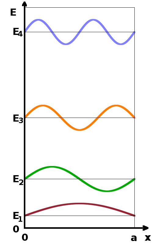
In order to determine the translational partition function, we can use the quantum-mechanical particle in a box model. In one dimension, it determines that the energy levels of a particle enclosed in a box of length $a$ are given by $$E_{\textrm{trans}}=\frac{n^2h^2}{8ma^2}\qquad,$$ where the energy levels are spaced in terms of the square of the quantum number, $n$, the mass of the particle is $m$, and $h$ stands for Planck's constant. The translational partition function is therefore $$z_{\textrm{trans}}=\sum_{n=1}^{\infty}\exp{\left(-\frac{n^2h^2}{8ma^2k_BT}\right)}\qquad.$$ Given that the energy levels are close together on an energy scale, we can replace the sum with an integral: $$z_{\textrm{trans}}\approx\int_n\exp{\left(-\frac{n^2h^2}{8ma^2k_BT}\right)}{\rm d}n\qquad.$$ With the substitution $$x=\sqrt{\frac{n^2h^2}{8ma^2k_BT}}$$ and its derivative $$\frac{{\rm d}x}{{\rm d}n}=\sqrt{\frac{h^2}{8ma^2k_BT}}$$ we can substitute ${\rm d}n$ in order to reduce the integral to a standard form, for which a known solution exists: $$\int_x{\rm e}^{-x^2}{\rm d}x=\frac{\sqrt{\pi}}{2}\qquad.$$ Therefore, the translational partition function becomes $$z_{trans}=\sqrt{2\pi mk_BT}\frac{a}{h}$$ in one dimension or, given that partition functions are multiplied together, $$z_{trans}=\left(2\pi mk_BT\right)^{\frac{3}{2}}\frac{V}{h^3}\qquad,$$ where $V=a^3$ is the volume in which the molecule can move around (i.e. the box).
In this derivation, we have transformed the partition function from a sum over all (infinitely many) states to a formula which requires no knowledge about any states in particular, just the system as a whole. This was achieved by replacing the sum with an integral (justifiable because states are packed closely together in energy) and solving the integral by reducing it to a standard form for which the solution is known. This can, in principle, be done for any partition function, including the ones for vibration, rotation and electronic excitation shown as sums below.
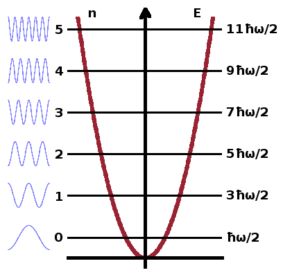
The vibrational partition function can be derived from the quantum-mechanical harmonic oscillator model, which gives the energy levels of an oscillator (i.e. a chemical bond between two atoms, represented as a spring with two attached masses) as $$E_{\textrm{vib}}=\left(m+\frac{1}{2}\right)\hbar\omega\qquad,$$ where $\omega$ is the angular frequency of the oscillation. The ½-term represents the zero-point energy of the system, i.e. the energy the system retains even at absolute zero temperature. This originates from the uncertainty principle of quantum mechanics - if the oscillation was to cease altogether, position and momentum could be known simultaneously at arbitrary precision.
The vibrational partition function is the sum of the Boltzmann terms of all energy levels: $$z_{\textrm{vib}}=\sum_{m=1}^{\infty}\exp{\left(-\frac{(m+\frac{1}{2})\hbar\omega}{k_BT}\right)}\qquad.$$ This can be simplified to avoid summing terms explicitly. To demonstate this, it is easiest to substitute $$x=\frac{\hbar\omega}{k_BT}\qquad,$$ so we have $$z_{\textrm{vib}}=\sum_m{\rm e}^{-x\left(m+\frac{1}{2}\right)}\qquad.$$ After multiplying both sides of the equation by ${\rm e}^{-x}$,
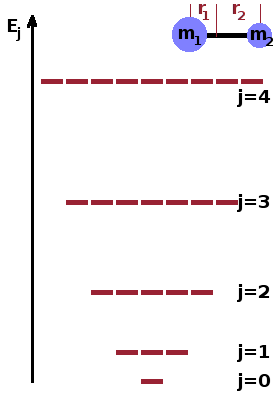
For simple diatomic linear molecules such as nitrogen, $\mathrm{N_2}$ or carbon monoxide, CO, the quantum mechanical rigid rotor model gives an adequate description of the rotational energy levels. It can be used to derive the rotational partition function in these cases. For more complex molecules, it may be necessary to consider rotations around several axis which may or may not co-incide with particular chemical bonds. For the rigid rotor, the energy levels are $$E_{\textrm{rot}}=\frac{j(j+1)h^2}{8\pi^2I}\qquad,$$ where $j$ is the rotational quantum number. As can be seen, there is no zero-point energy for rotational states. The distance of each atom from the centre of gravity of the molecule determines the moment of inertia, $I=mr^2$, of each atom. For each energy level, there exist several states (with different wave functions but identical energy). This is captured by the degeneracy, $g_j=2j+1$, i.e. the number of states at each energy increases rapidly as the quantum number increases. This must be taken into account when calculating the rotational partition function: $$z_{\textrm{rot}}=\sum_{j=0}^{\infty}(2j+1)\exp{\left(-\frac{j(j+1)h^2}{8\pi^2Ik_BT}\right)}\qquad.$$ Here, each Boltzmann term within the sum is weighted by its degeneracy.
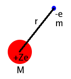
The
electronic partition function
is based on the simplest model of an atom developed by quantum mechanics, the
Statistically speaking, a system is in equilibrium if the distribution of its particles across energy levels conforms with the most probable macrostate. Therefore, if the statistical weight of the macrostate of a system is smaller than that of the most probable macrostate, particles will change levels until the system equilibrates towards the most probable configuration. Therefore, the statistical weight has the same function in statistical thermodynamics that entropy has in classical thermodynamics: it determines the direction of processes. There are a few mathematical differences though: While entropies are additive, statistical weights are multiplicative: $$S=S_1+S_2\qquad\textrm{but}\qquad\Omega=\Omega_1\Omega_2\qquad.$$ Since the logarithm of a product is the same as the sum of the logarithms of its factors, $$\color{grey}{\ln{xy}=\ln{x}+\ln{y}}\qquad,$$ entropy can be identified with the logarithm of the statistical weight. Boltzmann's constant is the constant of proportionality and provides the correct units, J/(mol K):
So far, we have assumed that we can distinguish different particles from one another. Classically, this is appropriate (although it may be cumbersome to do so given the large numbers involved). However, in quantum systems, this assumption isn't always applicable. The quantum statistics deal with that.