
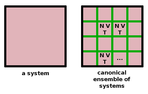
All of the particle statistics have been derived on the assumption that the particles to be distributed over energy levels do not interact. If they were to interact, we cannot be certain that each microstate would have the same probability, which is the fundamental assumption made in the derivation of the distribution functions. For interacting particles, we can obtain distribution functions by considering an ensemble of identical copies of the system and letting them all evolve and equilibrate separately. Alternatively, we can conceive of the one system being sliced up into many individual cells which can evolve separately. Depending on the kind of walls between the copies or cells of the system, three different types of ensemble are distinguished:
These are used under different sets of conditions, but the most generally used ensemble is the canonical ensemble, which is characterised by diathermal boundaries between the contributing systems, keeping them in thermal contact.
The fundamental idea of ensemble statistics is that time average equals ensemble average. We can therefore apply the same statistics to average a single snapshot of many identical systems as we would for multiple snapshots of a single system at different times. Since the particles cannot cross the boundaries separating the cells of the ensemble, interaction between the particles can be ruled out in this fashion.
The statistical weight of a distribution of an ensemble is calculated in the same way as a particle distribution function: $$\mathscr{\Omega}=\prod_i{\frac{\mathscr{N}!}{\mathscr{N}_i!}}\qquad,$$ where the number of instances, $\mathscr{N}$ and the total energy of ensemble, $\mathscr{E}$ substitute for the corresponding quantities in the Boltzmann distribution. We can find the most probable ensemble configuration and the ensemble partition function $$\mathscr{Z}=\sum_i\exp{\left(-\frac{\mathscr{E}_i}{k_BT}\right)}$$ in an exactly analoguous way.
Partition functions are the interface between quantum mechanics and thermodynamics. Different quantum mechanical models have been developed for different aspects of the behaviour of atoms and molecules such as translation, vibration, rotation, electronic excitation and magnetic interaction. Each model produces a series of energy levels and a partition function. Below are the rules for combining them. Energies are additive: $$E=\sum_i{E_i}\qquad,$$ while partition functions are multiplicative: $$Z=\sum_i\exp{\left(-\frac{E_i}{k_BT}\right)}=\prod_i z_i\qquad.$$ For distinguishable particles the system partition function is the product of the partition functions of the individual processes: $$Z=z^N\qquad.$$ For indistinguishable particles, we have to take into account that swapping two particles doesn't constitute a new microstate, so the system partition function reduces to $$Z=\frac{z^N}{N!}\qquad.$$
That concludes the second-year thermodynamics course. There will be more on the quantum-mechanical models supporting partition functions in the second-year quantum mechanics course (notes linked from a past edition of the module). Phase transitions and energy levels in atoms and molecules feature again in the third-year condensed matter and atomic and molecular physics modules.