
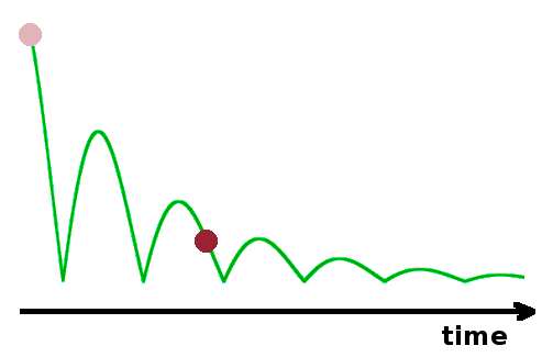

Work and heat are both forms of energy in transit. However, they are distinguished by their ordered or disordered nature, respectively. While atomic movements are facing in the same direction to the extent to which work is done, random atomic motions add up to heat. Although energy is conserved, the potential to extract work from a system diminishes during any real process. As a ball bounces off the ground, some of its kinetic energy is converted to heat through friction, diminishing its ability to work against gravity to rise from the ground. As a result, we can tell the direction of time by looking at the trajectory a bouncing ball has taken. This would even be the case if the floor is perfectly adiabatic: the heat generated would remain inside the system ball, but this amount of energy would no longer be available to propel the ball upwards.
The only kind of process during which no work becomes unavailable is a reversible process, i.e. a process in which all steps are infinitesimally small and occur infinitesimally slowly. The principle of microscopic reversibility entails that every step along the way can be undone without the need for any appreciable amount of energy to be transferred. Therefore no changes need to be made to the surroundings of the system in order to reverse the process. This implies that any reversible process must be quasi-static. However, quasi-static processes aren't necessarily reversible - if friction occurs, work is still converted to heat even if it happens infinitely slowly. Therefore, every real process is irreversible.
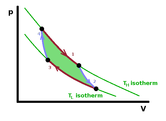
The Carnot engine is a hypothetical heat engine based on an entirely reversible cyclic process. The cycle consists of four separate steps as shown in the $pV$ diagram:
The engine operates a cycle between two isotherms at different temperature. The two isothermal steps are linked by adiabatic ones, where (by definition) no heat is exchanged; therefore the temperature must change (in the same way as it does in the adiabatic throttle experiment).
Carnot's theorem states that, for a given temperature difference,
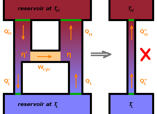
To demonstrate this, consider two Carnot engines coupled together back to back, i.e. the work done by the engine on the left is fed into the one on the right, which acts as a heat pump. If the Carnot heat pump were more efficient than the Carnot heat engine, it would pump more heat from the cold reservoir to the hot one than flows through the heat engine in the opposite direction. This would violate the Clausius statement of the Second Law. Since all processes are reversible, we could reverse the action of both engines, and the same argument would apply the other way. Thus, both engines must have the same efficiency if they are both reversible engines.
If only one of the engines is reversible, we need to consider separately what would happen if one of the engines was more efficient: If the irreversible heat engine was more efficient, it would take less heat from $T_H$ and dump less heat at $T_L$, again resulting in a Clausius violation since the reversible heat pump would transfer more heat up than flows down through the heat engine. On the other hand, if the irreversible heat pump was more efficient, then the amount of work, $W_{cyc}$, received from the reversible heat engine would allow it to transfer more heat from the reservoir at $T_L$ than is fed into it from the heat engine, again violating the Clausius statement. Therefore, either way, the reversible component must be the more efficient one.
Carnot's theorem is just another form of the Second Law.
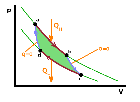
Given that all reversible processes operating between the same two temperatures are equally efficient, we can make arbitrary assumptions about the details of the system in order to calculate the reversible efficiency. It is easy to calculate the efficiency if the system contains an ideal gas since we know the relationship between the state variables in that case. Since the first step of the Carnot cycle is isothermal, the heat, $Q_H$, transferred from the hot reservoir equals the work done by the system during the isothermal expansion. By substituting the pressure according to the ideal gas law and integrating over the volume change, we have $$\begin{eqnarray} Q_H&=&W_{ab}\\ &=&\int_a^bp{\rm d}V\\ &=&\int_{V_a}^{V_b}{\frac{nRT_H}{V}{\rm d}V}\\ &=&nRT_H\ln\frac{V_b}{V_a}\qquad, \end{eqnarray}$$ and, in the same vein, the heat transferred from the system to the cold reservoir is $$Q_L=W_{cd}=nRT_L\ln\frac{V_d}{V_c}\qquad.$$ Note that $Q_L$ has a negative value (in line with the sign conventions introduced earlier) since $V_d\lt V_c$. To calculate the efficiency of a reversible engine, we can start from the definition of efficiency:
$$\eta_{rev}=1-\frac{|Q_L|}{Q_H}=1-\frac{\left|T_L\ln\frac{V_d}{V_c}\right|}{T_H\ln\frac{V_b}{V_a}} =1-\frac{T_L\ln\frac{V_c}{V_d}}{T_H\ln\frac{V_b}{V_a}}\qquad.\qquad\qquad\color{grey}{\left[\ln(x^a)=a\ln(x),\,\textrm{so}\,\ln(x^{-1})=-\ln(x)\right]}$$
Since the states b and c on the one hand and a and d on the other are adiabatically linked, the two volume ratios are the same, so the logarithms cancel out: $$\eta_{rev}=1-\frac{T_L}{T_H}\qquad.$$ Therefore, reversible efficiency depends only on the temperature gradient. This is an important finding because it allows us to use state variables in place of process variables: It doesn't matter how the reversible engine operates, the only information we need is the temperature at either end. This, together with Carnot's theorem, means that we can use the reversible cycle as a benchmark against which to compare real processes. For a real power station, for example, the temperature gradient between the boiler and the heat sink is still an important factor determining the efficiency of the process, but other losses within the power station will also contribute.
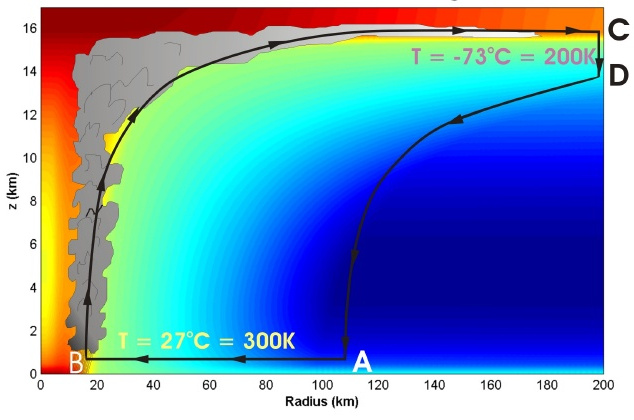
It has been suggested that tropical cyclones, including hurricanes, can be described as a reasonable approximation to a Carnot engine operating between two reservoirs, the sea and the stratosphere. The sea typically is at a temperature of about 300K, while the stratosphere boundary some 15km above is at around 200K.
The air flow begins as hot, humid air is drawn radially inward at sea level by the low-pressure system at the eye of the storm. Due to the contact with the sea reservoir, this is an isothermal process. This is followed by a rapid uplift in the eye wall, where the rotary wind speed is highest and the only way for the air mass to go is up. As this is a very fast upward movement, there is no time to equilibrate, and the process can be described approximately as adiabatic, i.e. no heat is lost from the air inside the eye wall. As the air mass hits the stratosphere boundary, it is put into contact with the cold reservoir of the stratosphere. The air can expand radially here, resulting in an air flow outward along the boundary. This is an isothermal process as the stratosphere has a practically unlimited capacity to take up heat from the storm while maintaining its own temperature. The final step is the down wind at the edge of the cyclone as the now cold air falls back to sea level. This is also a fast movement, which can be approximated as adiabatic.
Comparing this schematic of a tropical cyclone with the Carnot $p(V)$ diagram shows that the four steps of the Carnot cycle are all represented in the storm. The high-temperature isotherm is at sea level, while the cold isotherm is at the stratosphere boundary. The isotherms are connected by (near) adiabatic expansion and compression steps. The work done by the storm is enclosed by the loop in the $p(V)$ diagram and manifests itself as horizontal wind and friction (i.e. damage to the ground and structures over land).
It doesn't matter how a reversible process operates since all reversible processes operating between the
same two reservoirs are equally efficient. Therefore, we can compare the heat transferred in a real,
irreversible process with the heat that would have been transferred under reversible conditions. This
should provide a measure of how far from the ideal an actual process is. It is best to normalise the
heat transferred by the temperature at which this happens so that we can compare systems in contact with
different reservoirs:
Heat transferred reversibly, divided by the temperature at which it is transferred, is a state variable.
This quantity is known as
entropy, $S$, in J/K,
and is defined as the heat transferred in a reversible process, divided by the temperature at which this happens:
$${\rm d}S=\frac{{\rm d}Q_{rev}}{T}\qquad.$$
The definition doesn't require that heat is actually transferred reversibly. Entropy is a state variable,
and its change corresponds to the heat that would be transferred if the transfer were reversible.
As it is a state variable, we can see that the entropy change during any cycle (reversible or otherwise)
must be zero as the initial and final states are the same:
$$\Delta S=S_f-S_i=\int_i^f{\frac{Q_{rev}}{T}}{\rm d}T\overset{!}{=}0$$
for any cycle.
It follows that the difference between the actual heat transferred (divided by temperature) and the change in entropy during any process,
$$\left(\frac{{\rm d}Q}{T}-{\rm d}S\right)\qquad,$$
is a
measure of irreversibility.
Example:
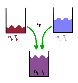
$n_H$=3mol, $T_H$=90oC
$n_L$=7mol, $T_L$=10oC
$c_p$=72J/(mol K)
As an example of how to calculate entropy changes during irreversible processes, consider the process of mixing hot and cold water. In order to do this, we need to calculate the heat transferred away from the hot molecules and to the cold molecules during the actual, spontaneous mixing process and compare it to the heat that would have been transferred if the mixing could be undone.
First, we need to work out the final temperature of the mixture. The heat transferred from the hot molecules is $$Q_H^{irv}=n_Hc_p(T_H-T_f)\qquad,$$ and the heat transferred to the cold molecules is $$Q_L^{irv}=n_Lc_p(T_f-T_L)\qquad.$$ Naturally, they have to be the same (neglecting any loss of heat to the surroundings): $$Q_H=Q_L$$ $$n_Hc_p(T_H-T_f)=n_Lc_p(T_f-T_L)\qquad.$$ This we can solve for $T_f$:
$$T_f=\frac{n_HT_H+n_LT_L}{n_L+n_H}=\frac{\textrm{3mol}\,\textrm{363K+7mol}\,\textrm{283K}}{\textrm{3mol+7mol}}=\textrm{307K}=\textrm{34}^o\textrm{C}\qquad.$$
Next we calculate the entropy change separately for the molecules in the hot sample and those in the cold sample. The entropy change to the hot water is $$\Delta S_H=\int_i^f{\frac{{\rm d}Q_{rev}}{T}}\qquad.$$ This time, we don't just take the difference in temperatures between the initial and the final state but rather integrate all along the way in order to trace the process reversibly in infinitesimal steps. Neglecting the very small temperature dependence of the heat capacity for the purposes of this illustration, the integral simplifies to
$$\Delta S_H=n_Hc_p\int_{T_H}^{T_f}{\frac{1}{T}}{\rm d}T=n_Hc_p\ln{\frac{T_f}{T_H}}= \textrm{3mol}\,72\frac{\rm J}{\rm mol K}\ln{\frac{307{\rm K}}{363{\rm K}}}=-36.2\,\textrm{J/K}\qquad.$$
Remember to convert the temperatures to Kelvins - using degrees Celsius in fractions causes errors because the conversion is an offset rather than a factor.
Evidently, the entropy of the hot water molecules is reduced in the cooling process.
In the same vein, we can calculate the entropy change of the cold water: $$\Delta S_L=n_Lc_p\ln{\frac{T_f}{T_L}}=+41.0\,\textrm{J/K}$$ The entropy of the molecules from the cold sample increases.
Finally, we can calculate the entropy change of the system as a whole, the entropy of mixing: $$\Delta_{mix}S=\Delta S_L+\Delta S_H=+4.8\,\textrm{J/K}\qquad.$$
A note on notation: The subscript 'mix' is appended to the $\Delta$ sign, indicating that it refers to the process of mixing, while the subscripts 'L' and 'H' are appended to the variable $S$ as they refer to the two initial states from which the process starts.
The net change in entropy of the system water as a consequence of mixing the two portions is therefore positive.
It is possible that the entropy of a system decreases during a process. In this case, the system becomes more
ordered and its potential to do work increases. However, this must come at the expense of an increase in
entropy in the surroundings.
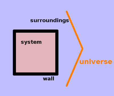
The entropy of the universe increases during any irreversible process.
In this statement, the universe is taken to mean the system and its surroundings taken together:
$$\Delta S_{univ}=\Delta S_{syst}+\Delta S_{surr}$$
It is a fourth way of phrasing the Second Law of Thermodynamics.
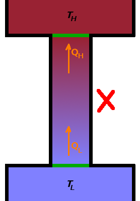
To demonstrate this, calculate the entropy change at the hot and cold end of a heat pump violating the
Clausius statement:
$$\Delta S_H=\frac{Q_{rev}}{T_H}$$
$$\Delta S_L=-\frac{Q_{rev}}{T_L}$$
Given that $T_H$ is larger than $T_L$, the entropy of the universe would decrease in such a device:
$$\Delta S_{univ}=Q_{rev}\left(\frac{1}{T_H}-\frac{1}{T_L}\right)\lt 0\qquad.$$
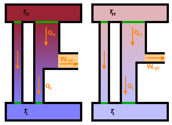
Two finite heat stores in thermal contact with each other will eventually equilibrate, i.e. their temperatures approach each other as time passes (indicated by the direct flow of heat from $T_H$ to $T_L$ in the Figure). A heat engine operating between these two heat stores will therefore operate on a gradually diminishing thermal gradient and, as a result, become progressively less efficient. The reduced work output, $W_{cyc}$, of the heat engine corresponds to an increase of entropy across the system as a whole (incorporating both the hot and cold heat stores). Work becomes unavailable as entropy increases. As the heat engine becomes less efficient, it dumps more heat into the cool heat store, exacerbating the deterioration of the thermal gradient.
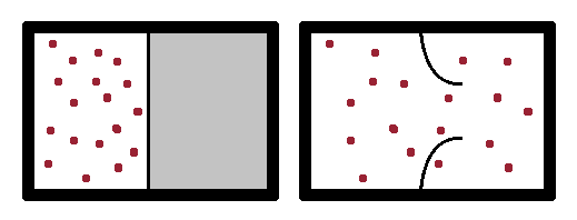
In a spontaneous process, such as spontaneous expansion of a gas by bursting a membrane enclosing it, the gas atoms suddenly have more space to spread out, their mean distance and the density of the configuration decrease. Since it is very unlikely that all atoms congregate in the same part of the enlarged volume, the increase in available volume increases the disorder of the system and therefore its entropy. As the pressure of the gas is now lower, its potential to do work is reduced.
We have introduced entropy as a differential, i.e. in terms of how much it changes during a process:
$${\rm d}S=\frac{{\rm d}Q_{rev}}{T}$$
However, entropy is a state variable, so the question arises what the absolute entropy of a state might be.
As in the case of the mixing example above, we can calculate the change of entropy over a range of temperatures
by integrating the ratio of heat capacity over temperature:
$$S=S_0+\int_0^T\frac{c_p}{T}{\rm d}T$$
provided we know (or can work out) the entropy $S_0$ at the lower limit of the integral. The
Third Law of Thermodynamics
provides that anchor point:
The entropy of any perfect crystal at T=0K is zero.
This has been concluded from measurements of the heat capacity at very low temperatures, where an
asymptotic
approach to zero was found. It is interesting to note that the Third Law applies to any perfect
(i.e. defect-free) crystal structure, even for materials which have several
polymorphs
(i.e. different crystal structures with the same composition).
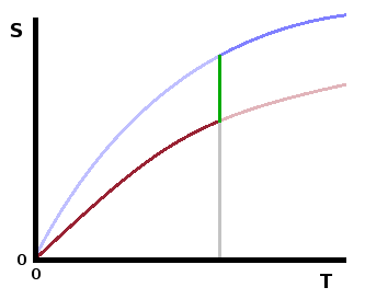
At temperatures above zero, the entropies of the different forms will be different, but this difference
diminishes as the zero point is approached.
Phase transitions
occur between polymorphs at specific temperatures (in the same way that melting and boiling points are
defined temperatures). Here the latent heat of the transition overcomes the product $T\Delta S$ between
the entropy curves of the two polymorphs involved.
The Third Law also defines the origin of the Kelvin temperature scale: Since the entropies of all perfect crystal structures converge on zero as absolute zero temperature is approached, there can be no lower temperatures as there is no entropy left that could be taken out of the system.
The First Law describes the internal energy as the sum of heat and work exchanged: $${\rm d}U={\rm d}Q+{\rm d}W\qquad.$$ In addition, we have introduced enthalpy by taking into account expansion work explicitly: $$H=U+pV\qquad.$$ If we are interested in the potential of the system to do work, we can subtract the entropy of the system from these energies since it determines the amount of energy that has become unavailable due to the disorder contained in the system. Entropy itself is not an energy; therefore it is necessary to multiply it by the temperature. Applying the entropy term, $TS$, to the internal energy and the enthalpy, respectively, defines the free energy or Helmholtz function, $A$, and the free enthalpy or Gibbs function, $G$: $$A=U-TS\qquad G=H-TS\qquad.$$
When considering reversible changes and expansion work, the First Law can be written in terms of temperature, entropy, pressure and volume: $${\rm d}U={\rm d}Q+{\rm d}W=T{\rm dS}-p{\rm d}V\qquad.$$ We can differentiate the definition of enthalpy and substitute ${\rm d}U$ in it: $${\rm d}H={\rm d}U+p{\rm d}V+V{\rm d}p=T{\rm d}S+V{\rm d}p\qquad.$$ Similarly, a differential form of the Helmholtz energy is $${\rm d}A={\rm dU}-T{\rm d}S-S{\rm d}T=-p{\rm d}V-S{\rm d}T\qquad,$$ and for the Gibbs enthalpy, we have $${\rm d}G={\rm d}H-T{\rm d}S-S{\rm d}T=V{\rm d}p-S{\rm d}T\qquad.$$ To summarise, this produces the four differential energies, each consisting of a TS and a pV term:
$${\rm d}U=T{\rm dS}-p{\rm d}V\qquad{\rm d}H=T{\rm d}S+V{\rm d}p\qquad{\rm d}A=-S{\rm d}T-p{\rm d}V\qquad{\rm d}G=-S{\rm d}T+V{\rm d}p$$
These four differential energies enable us to establish relationships between state variables. For example, temperature features in the first term of both the ${\rm d}U$ and the ${\rm d}H$ equations. If we choose conditions in which the other term is zero (i.e. constant volume, ${\rm d}V=0$, or constant pressure, ${\rm d}p=0$, respectively), we can bring the entropy differential ${\rm d}S$ over on the left-hand side and get two independent relationships equating to temperature: the change of internal energy with entropy at constant volume, $\left.\frac{\partial U}{\partial S}\right|_V$, and the change of enthalpy with entropy at constant pressure, $\left.\frac{\partial H}{\partial S}\right|_p$. Similar pairs of relationships can be found for pressure, entropy, and volume from the other three differential energy formulae:
$$ T= \left.\frac{\partial U}{\partial S}\right|_V= \left.\frac{\partial H}{\partial S}\right|_p\qquad p=-\left.\frac{\partial U}{\partial V}\right|_S=-\left.\frac{\partial A}{\partial V}\right|_T\qquad S=-\left.\frac{\partial A}{\partial T}\right|_V=-\left.\frac{\partial G}{\partial T}\right|_p\qquad V= \left.\frac{\partial H}{\partial p}\right|_S= \left.\frac{\partial G}{\partial p}\right|_T $$
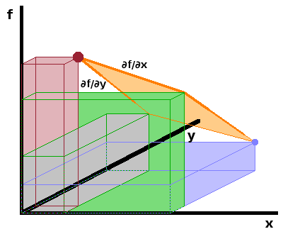
We can take this a step further and analyse the mixed second derivatives obtained by differentiating each of the partial differentials by the state variable kept constant so far. This utilises Schwarz's theorem, which says that the order in which a function $f(x,y)$ of several variables is differentiated is immaterial: $$\frac{\partial^2f}{\partial x\partial y}=\frac{\partial^2f}{\partial y\partial x}$$ as long as all first partial derivatives are themselves differentiable. As this condition is fulfilled for all state variables, we find $$\frac{\partial T}{\partial V}=\frac{\partial^2U}{\partial S\partial V}=\frac{\partial^2U}{\partial V\partial S}=-\frac{\partial p}{\partial S}$$ using the first differentials derived above for temperature and pressure, respectively. This is one of the Maxwell relations, and the full set can be derived analoguously:
$$ \left.\frac{\partial T}{\partial V}\right|_S=-\left.\frac{\partial p}{\partial S}\right|_V\qquad \left.\frac{\partial T}{\partial p}\right|_S= \left.\frac{\partial V}{\partial S}\right|_p\qquad \left.\frac{\partial S}{\partial V}\right|_T= \left.\frac{\partial p}{\partial T}\right|_V\qquad \left.\frac{\partial S}{\partial p}\right|_T=-\left.\frac{\partial V}{\partial T}\right|_p $$
The last of these is particularly useful since it substitutes a differential that is impossible to measure (change of entropy with pressure) with one that is easily measured (change of volume with temperature). The latter is essentially the volumetric thermal expansion coefficient, $\alpha=\frac{1}{V}\frac{{\rm d}V}{{\rm d}T}$.
To demonstrate the utility of this, we can look to a simple application: reversible isothermal compression. For a reversible process, $${\rm d}Q=T{\rm d}S\qquad.$$ State variables are dependent on each other, and we can express entropy as a state function, $S(p,T)$ of the independent variables temperature and pressure, and take its total differential: $${\rm d}S=\left.\frac{\partial S}{\partial T}\right|_p{\rm d}T+\left.\frac{\partial S}{\partial p}\right|_T{\rm d}p\qquad.$$ The heat transferred in the isothermal compression experiment is then $${\rm d}Q=T\left.\frac{\partial S}{\partial p}\right|_T{\rm d}p\qquad.$$ Entropy is difficult to measure, but we can avoid it by substituting one of the Maxwell relations and the thermal expansion coefficient: $${\rm d}Q=-T\left.\frac{\partial V}{\partial T}\right|_p{\rm d}p=-\alpha TV{\rm d}p$$ Finally, integrate to find the total heat transferred in the process: $$Q=-\int\alpha TV{\rm d}p\approx -\alpha TV\Delta p\qquad,$$ where the final step neglects the small pressure dependence of the thermal expansion coefficient and the compressibility of the material (reasonably for condensed phases, but clearly not valid if the medium were a gas).
The Maxwell relations give us a host of possible substitutions to replace quantities that would be difficult to measure with others that are more accessible. They link all the state variables to each other and allow us to calculate every aspect of a system in equilibrium provided we know the values of two independent state variables. We can therefore plot any state variable as a function of two other state variables, producing a phase diagram.