
The Maxwell relations establish how the different state variables depend on each other. A graphical representation showing these relationships is called a phase diagram. It shows the conditions under which a material exists in a particular state of matter such as solid, liquid or gas. A phase is a material in a uniform state and with a uniform composition. Its intensive state variables are homogeneous within its boundaries but may change abruptly at the boundary. A phase needn't be contiguous - several ice cubes in a glass of water form a single phase of solid, crystalline water. Phase diagrams always represent materials in thermodynamic equilibrium.
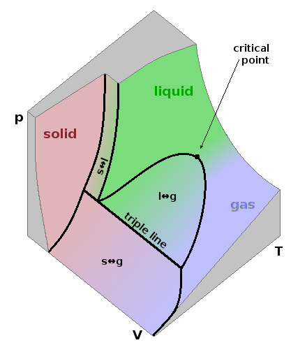
Any of the state variables (pressure, temperature, but also entropy or enthalpy...) can be shown on the axes of a phase diagram. Given that each state variable can be expressed as a state function depending on each of the other state variables, a phase diagram can only ever show a subset of this multi-dimensional parameter space. The three-dimensional $pVT$ diagram shown is an example of such a sub-set. It contains a highly structured curved surface representing the value of (any) one of the three state variables pressure, (molar) volume and temperature as a function of the other two. The figure shows a cube segment of the parameter space, with each of the three co-ordinate axes truncated. The function surface is shown in colours representing the three phases solid (red), liquid (green) and gas (blue). It contains both single-phase regions, where only one phase is present, and mixed-phase regions separating pairs of single-phase regions, where a material of a given composition exists in two forms concurrently. Within the two-phase regions, the material undergoes phase transitions: fusion (melting, s$\leftrightarrow$l) between solid and liquid, vapourisation (boiling, l$\leftrightarrow$g) between liquid and gaseous, and sublimation (s$\leftrightarrow$g) directly between solid and gaseous. Within these two-phase regions, the material is gradually transferred from one state to another, i.e. the relative amount of the two phases changes gradually. For example, when compressing a gas, a few drops of condensation form at first as we enter the two-phase region. Gradually, more and more of the gas turns into a boiling liquid until the pressure is high enough for boiling to cease, leaving behind a single-phase liquid.
The slopes surrounding the fusion region are much steeper than those surrounding the vapourisation region because condensed phases have a much lower compressibility than a gas. The triple line separates the sublimation region from the fusion and vapourisation regions. Along this line, all three phases co-exist. The triple line is exactly parallel to the volume axis, so all points along it share the same pressure and temperature.
The vapourisation region narrows as the temperature increases, ending at the critical point at its apex. Beyond this point, there is no phase transition between liquid and gas, i.e. the two phases merge into a single fluid phase which could be seen as a "dense gas" with unusually strong inter-molecular interactions or a highly disordered liquid where inter-molecular forces are weak and transient compared to those of a normal liquid. Such supercritical fluids have important applications in industrial drying and purification processes. Critical points aren't observed in the other two-phase regions. Theoretical studies argue that there cannot generally be critical points involving crystalline solids on symmetry grounds while considering that they can occur in systems involving less ordered solids.
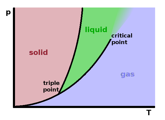
It is usually easier to work with two-dimensional phase diagrams. These are projections of the $pVT$ diagram onto one of the sides of its reference frame. The most common phase diagrams are $pT$ diagrams and, particularly useful for gases, $pV$ diagrams. Of course any two-dimensional representation of a complex three-dimensional shape will suffer some distortions, so care is needed when using them to avoid erroneous conclusions.
The diagram shows an approximate projection of the $pVT$ cube onto the $pT$ plane. It correctly represents the triple line as a unique triple point since the line is parallel to the volume axis. The two mixed-phase regions show as phase boundary lines. It is important to note that these lines are not isochores (i.e. the molar volume changes as one moves along the line). This is a significant distortion since the mixed-phase surfaces aren't in fact oriented parallel to the volume axis. The end of the vapourisation line in the critical point only applies to one particular molar volume value.
The phase equilibrium of the mixed-phase regions is driven by the Gibbs enthalpy of the phase mixture: $$G=x_1G_1+x_2G_2\qquad,$$ where $x_i$ are the molar fractions of the two phases and $G_i$ their Gibbs enthalpies. The equilibrium condition requires that the total Gibbs enthalpy remains unchanged: $${\rm d}G=G_1{\rm d}x_1+G_2{\rm d}x_2\overset{!}{=}0\qquad.$$ Since $$G_i=H_i-TS_i\qquad,$$ changing the temperature will change the entropy contribution to the Gibbs enthalpy, and the molar fractions have to balance this out to maintain the overall Gibbs enthalpy.
This is summarised by Gibbs's phase rule: If $P$ is the number of phases present in a system consisting of $C$ components (chemically distinct species), then the number $F$ of degrees of freedom, i.e. of intensive state variables that can be varied independently of each other, is $$F=C-P+2\qquad.$$
In a single-component system (such as those shown in the phase diagrams in this box: $C=1$), this leaves two degrees of freedom within each single-phase region: temperature and pressure can be changed independently without encountering phase separation. In the mixed-phase regions, there are two phases present, leaving only one degree of freedom: if the temperature changes, the pressure has to follow (or vice versa), otherwise we'll drop off the line into one of the adjacent single-phase regions. At the triple point, no degrees of freedom are left, and any change to pressure or temperature will cause at least one of the phases to vanish. The phase rule only applies to intensive state variables (ones that are uniform, such as temperature, rather than cumulative, such as volume). This is the reason why the triple line must be parallel to the volume axis in the $pVT$ diagram - it is the only extensive variable in this phase diagram.
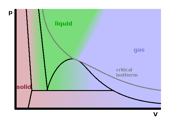
The diagram on the right summarises the relationship between pressure and volume. It shows a projection of the $pVT$ cube onto its $pV$ face, so the black lines shown are not isotherms (with the exception of the triple line, for the reasons discussed above). The three mixed-phase regions are evident. Since the change of volume with pressure is the compressibility of a material, it is clear that the slopes separating the condensed phases from each other must be much steeper than those involving a gas. Clearly, everything else being equal, the volume must decrease when the pressure is increased; therefore we should expect all slopes to be negative. The positive slope at the wet end of the vapourisation zone is possible because the temperature changes as well. At any particular temperature, we would cut through the two-phase region horizontally while liquid is turned into gas, increasing the occupied volume while keeping the pressure constant. The grey line shown is the critical isotherm, i.e. the isotherm running through the critical point at the apex of the vaporisation region. At this temperature, the slope of the curve decreases monotonously, with a saddle point at the critical pressure.
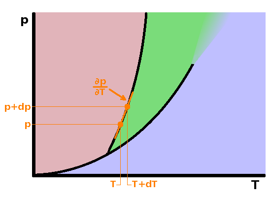
For most materials, the slopes of all phase transition lines in a $pT$ diagram are positive, but how steep exactly are they expected to be? To find out the slope of these curves, we need to consider that the common property of all points along the line is that there is a phase equilibrium under the specific conditions at each point along the line, i.e. that both phases coexist. The equilibrium condition is that the Gibbs enthalpy of both phases is the same: $$G_1(p,T)=G_2(p,T)\qquad.$$ This is true of any point along the transition line, including a second point only removed from the first by infinitesimal increments of temperature and pressure: $$G_1(p+{\rm d}p,T+{\rm d}T)=G_2(p+{\rm d}p,T+{\rm d}T)\qquad.$$ Using Taylor expansion on the second equation, we find the Gibbs enthalpy of the second point by moving, separately, an infinitesimal amount along the $p$ and $T$ axes, multiplying the increment ${\rm d}p$ by the slope of the function in that direction, $\left.\frac{\partial G}{\partial p}\right|_T$, and the same along the $T$ axis. The Taylor expansion includes higher order terms considering the second and higher derivatives as well, which are neglected here: $$G_1(p,T)+\left.\frac{\partial G_1}{\partial p}\right|_T{\rm d}p+\left.\frac{\partial G_1}{\partial T}\right|_p{\rm d}T =G_2(p,T)+\left.\frac{\partial G_2}{\partial p}\right|_T{\rm d}p+\left.\frac{\partial G_2}{\partial T}\right|_p{\rm d}T\qquad.$$ The first terms on each side are the Gibbs enthalpies of both phases at the original point. Since they have to be equal due to the equilibrium condition, this leaves $$\left.\frac{\partial G_1}{\partial p}\right|_T{\rm d}p+\left.\frac{\partial G_1}{\partial T}\right|_p{\rm d}T =\left.\frac{\partial G_2}{\partial p}\right|_T{\rm d}p+\left.\frac{\partial G_2}{\partial T}\right|_p{\rm d}T\qquad.$$ Now separate the ${\rm d}p$ and ${\rm d}T$ terms on the left and right side of the equation, respectively: $$\left(\left.\frac{\partial G_1}{\partial p}\right|_T-\left.\frac{\partial G_2}{\partial p}\right|_T\right){\rm d}p =\left(\left.\frac{\partial G_2}{\partial T}\right|_p-\left.\frac{\partial G_1}{\partial T}\right|_p\right){\rm d}T\qquad.$$ As developed when introducing the four energy state variables $U$, $H$, $G$ and $A$, the definition of the Gibbs enthalpy is $$G=H-TS=U+pV-TS\qquad,$$ and its differential is $${\rm d}G=V{\rm d}p-S{\rm d}T\qquad.$$ By keeping one of the differential state variables constant, we can drop one term from the right and bring the other differential over to the left, leaving equations showing how volume and entropy are derivatives of the Gibbs enthalpy: $$V=\left.\frac{\partial G}{\partial p}\right|_T\qquad\textrm{and}\qquad S=-\left.\frac{\partial G}{\partial T}\right|_p\qquad.$$ This we can insert into the brackets above: $$(V_1-V_2){\rm d}p=(S_1-S_2){\rm d}T\qquad,$$ and bringing the differentials together on one side produces the slope of pressure with temperature, which we were looking for: $$\frac{\partial p}{\partial T}=\frac{\Delta S}{\Delta V}\qquad,$$ where $\Delta S$ and $\Delta V$ are the entropy and (molar) volume differences between the two phases in equilibrium - not a differential but rather a step change at the phase boundary. Given that the latent heat, L, under isobaric conditions is $$L=T\Delta S\qquad,$$ we get the Clausius-Clapeyron equation for the slope of a phase transition line in the $pT$ diagram:
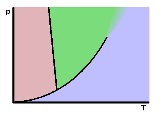
Since both $L$ and $T$ are positive, the Clausius-Clapeyron equation shows that the slope will be positive if the volume difference between the two phases is positive. This will always be the case between a condensed phase on one side and a gas on the other. For most materials, the melting line is also positive since the density of melts is typically lower (i.e. their volume larger) than that of the solid. Water (and a few other materials) shows an anomaly in that the density of ice is lower than that of liquid water, resulting -in line with the Clausius-Clapeyron equation- in a negative slope of the melting boundary.
Under the (rather crude) assumption that the gas phase can be modelled as an ideal gas, we can calculate the shape of the vapourisation line. $$pV=RT$$ In this case, the Clausius-Clapeyron equation can be simplified by considering that the molar volume of the condensed phase is much smaller than that of the gas, i.e. $\Delta V\approx V_g$ and can be substituted by the ideal gas law, $V_g=\frac{RT}{p}$: $$\frac{{\rm d}p}{{\rm d}T}=\frac{L}{T\Delta V}\approx\frac{L}{TV_g}\approx\frac{Lp}{RT^2}\qquad.$$
Phase transitions such as melting, boiling and submlimation are known as first-order phase transitions. These are phase transitions which have a clear latent heat associated with them. There are other phase transitions for which there is no latent heat, or at least it is too small to be observed experimentally. These are second-order phase transitions. First and second order phase transitions can be distinguished by the dependence of their Gibbs enthalpy and its derivatives as the temperature rises above the transition temperature.
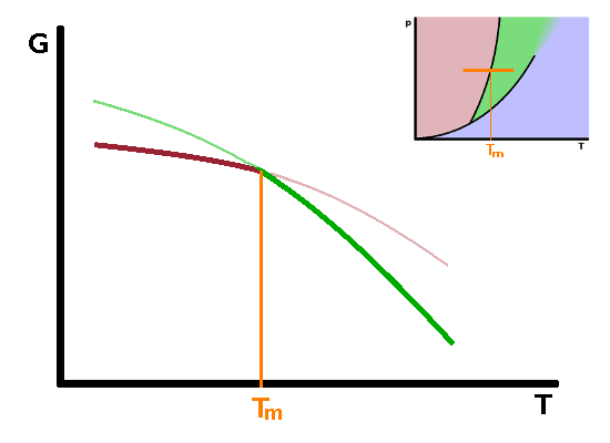
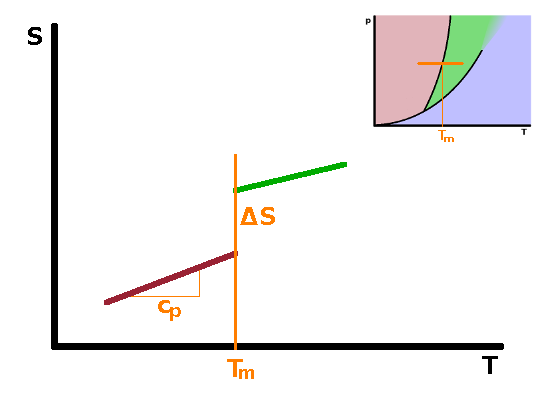
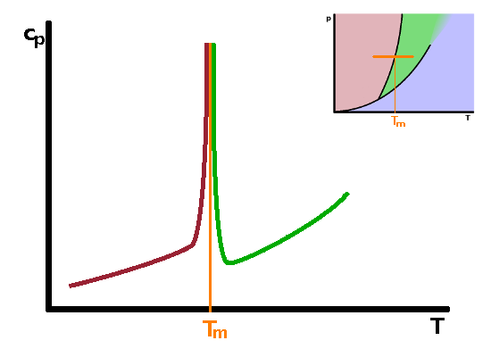
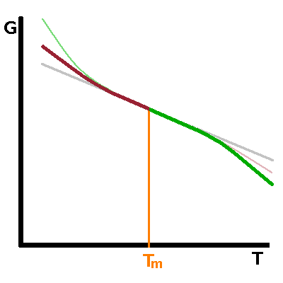
From the differential form of the Gibbs enthalpy, $${\rm d}G=V{\rm d}p-S{\rm d}T\qquad,$$ we see that the derivative of the Gibbs enthalpy with respect to temperature under isobaric conditions is the negative entropy: $$\left.\frac{\partial G}{\partial T}\right|_p=-S\qquad.$$ Since entropy increases with temperature, the slope of $G(T)$ must be negative for both phases involved in a phase transition. At the phase transition temperature, the Gibbs enthalpies of both phases are the same, so the two curves cross over each other at that point, in other words the slope of the Gibbs enthalpy with temperature changes abruptly at the transition as we move from one phase across the phase boundary line into the other phase. Plotting the entropy against temperature therefore shows a discontinuity - a step corresponding to the latent heat. Since the entropy is defined as $$S=\int\frac{c_p}{T}{\rm d}T\qquad,$$ the slope of the entropy curve with temperature is the heat capacity $c_p$: $$\frac{\partial S}{\partial T}=\frac{c_p}{T}\qquad.$$ Therefore the heat capacity is related to the second derivative of the Gibbs enthalpy with respect to temperature: $$\left.\frac{\partial^2G}{\partial T^2}\right|_p=-\left.\frac{\partial S}{\partial T}\right|_p=-\frac{c_p}{T}$$ As there is a step in the first derivative, there must be a singularity in the second derivative: the heat capacity shoots up to infinity immediately before the phase transition and returns to levels similar to those before the transition immediately after the transition has occurred. The same behaviour (step in the first derivative, singularity in the second) is observed for derivatives of the Gibbs enthalpy with respect to other state variables.
In second-order phase transitions, there is no latent heat, therefore no step in first derivatives of the Gibbs enthalpy such as entropy. As a result, the Gibbs enthalpy changes continuously rather than abruptly at the phase transition. The entropy behaves much like the Gibbs enthalpy does in a first-order transition, i.e. its slope changes abruptly. Its derivative, the heat capacity, therefore has a step similarly to that observed in the entropy in a first-order transition. Examples of such second-order transitions include transitions between different magnetic states of matter or some crystallographic transitions between different crystalline solid phases.
Of course, it is not always possible to be certain that there is no latent heat if none can be measured. It could just be the case that the measurement is not precise enough, or the system is not quite in thermal equilibrium during the measurement. This has led to the suggestion that there may in fact not be any truly second-order transitions, just ones with immeasurably small latent heat.
The Clausius-Clapeyron equation links the slope of a phase transition line in the $pT$ diagram with the change of entropy and volume at the phase transition: $$\frac{\partial p}{\partial T}=\frac{\Delta S}{\Delta V}\qquad.$$ However, for second-order transitions, we have seen that there is no entropy change, and since the slope cannot be zero, there cannot be a volume change in these cases either. Therefore, the Clausius-Clapeyron equation is useless when it comes to second-order phase transitions. However, the same method of derivation can be used based on the fact that the entropy and the volume of both phases must be the same in these cases. These lead to the first and second Ehrenfest equations for the slope of $pT$ phase boundaries in second-order phase transitions. The table shows the derivation of the Clausius-Clapeyron equation again and the analogous steps needed to derive the Ehrenfest equations:
| Clausius-Clapeyron | Ehrenfest 1 | Ehrenfest 2 |
|---|---|---|
| $$G_1(p,T)=G_2(p,T)$$ | $$S_1(p,T)=S_2(p,T)$$ | $$V_1(p,T)=V_2(p,T)$$ |
| $$G_1(p+{\rm d}p,T+{\rm d}T)\\\qquad=G_2(p+{\rm d}p,T+{\rm d}T)$$ | $$S_1(p+{\rm d}p,T+{\rm d}T)\\\qquad=S_2(p+{\rm d}p,T+{\rm d}T)$$ | $$V_1(p+{\rm d}p,T+{\rm d}T)\\\qquad=V_2(p+{\rm d}p,T+{\rm d}T)$$ |
| $$\left(\left.\frac{\partial G_1}{\partial p}\right|_T-\left.\frac{\partial G_2}{\partial p}\right|_T\right){\rm d}p\\ \qquad=\left(\left.\frac{\partial G_2}{\partial T}\right|_p-\left.\frac{\partial G_1}{\partial T}\right|_p\right){\rm d}T$$ | $$\left(\left.\frac{\partial S_1}{\partial p}\right|_T-\left.\frac{\partial S_2}{\partial p}\right|_T\right){\rm d}p\\ \qquad=\left(\left.\frac{\partial S_2}{\partial T}\right|_p-\left.\frac{\partial S_1}{\partial T}\right|_p\right){\rm d}T$$ | $$\left(\left.\frac{\partial V_1}{\partial p}\right|_T-\left.\frac{\partial V_2}{\partial p}\right|_T\right){\rm d}p\\ \qquad=\left(\left.\frac{\partial V_2}{\partial T}\right|_p-\left.\frac{\partial V_1}{\partial T}\right|_p\right){\rm d}T$$ |
| $$V=\left.\frac{\partial G}{\partial p}\right|_T$$ and $$S=-\left.\frac{\partial G}{\partial T}\right|_p$$ | Here we use the definition of entropy to express $\frac{\partial S}{\partial T}$ in terms of the heat capacity, $c_p$. The other differential can be replaced (according to one of the Maxwell relations) by the definition of the thermal volume expansion coefficient, $\alpha$. $$c_p=T\left.\frac{\partial S}{\partial T}\right|_p$$ and$$\alpha=\frac{1}{V}\left.\frac{\partial V}{\partial T}\right|_p$$ | Here we can substitute the definitions of the compressibility, $\kappa$, and the thermal volume expansion coefficient, $\alpha$. $$\kappa=-\frac{1}{V}\left.\frac{\partial V}{\partial p}\right|_T$$ and $$\alpha=\frac{1}{V}\left.\frac{\partial V}{\partial T}\right|_p$$ |
| $$\frac{\partial p}{\partial T}=\frac{\Delta S}{\Delta V}$$ | $$\frac{\partial p}{\partial T}=\frac{\Delta c_p}{TV\Delta\alpha}$$ | $$\frac{\partial p}{\partial T}=\frac{\Delta\alpha}{\Delta\kappa}$$ |
In all of these equations, the $\Delta$s refer to the differences in the respective properties between the two
phases involved in the phase transition. Note that the Clausius-Clapeyron equation applies only to
first-order transitions (since $\frac{\Delta S}{\Delta V}$ is indeterminate otherwise) while the Ehrenfest
equations apply only to second-order transitions since the assumptions
($\Delta V=0$ and $\Delta S=0$,
respectively) don't hold for first-order transitions.
As another example of an application of the thermodynamic relationships, we can calculate the difference between the heat capacities of an arbitrary material under isobaric and isochoric conditions. In many cases it is easier to measure under one set of conditions which are more straightforward to realise experimentally and work out the properties of a system under different conditions by using thermodynamic relationships.
To start, consider that entropy is a state function depending on two other state variables, e.g. temperature and volume: $$S(T,V)\qquad.$$ We can determine its total differential by differentiating separately by each of the independent variables and multiplying the result with a differential of the respective variable: $${\rm d}S=\left.\frac{\partial S}{\partial T}\right|_V{\rm d}T+\left.\frac{\partial S}{\partial V}\right|_T{\rm d}V\qquad.$$ By dividing this equation by the temperature differential ${\rm d}T$ and multiplying it by the temperature itself, we have $$T\left.\frac{\partial S}{\partial T}\right|_p=T\left.\frac{\partial S}{\partial T}\right|_V+T\left.\frac{\partial S}{\partial V}\right|_T\left.\frac{\partial V}{\partial T}\right|_p\qquad,$$ which brings the equation into a form where we can substitute the two heat capacities due to the relationship between differential entropy and heat capacity under isobaric and isochoric conditions, respectively: $${\rm d}S=\frac{c_{p,v}}{T}{\rm d}T\qquad.$$ With this substitution, the equation becomes $$c_p=c_v+T\left.\frac{\partial S}{\partial V}\right|_T\left.\frac{\partial V}{\partial T}\right|_p\qquad,$$ making it clear that the difference between the two heat capacities is an additional term.
Unfortunately, the change of entropy with volume under isothermal conditions is very difficult to measure. However, one of the Maxwell relations allows us to substitute it with the temperature dependence of pressure under isochoric conditions: $$\left.\frac{\partial S}{\partial V}\right|_T=\left.\frac{\partial p}{\partial T}\right|_V$$ so that the equation becomes $$c_p=c_v+T\left.\frac{\partial p}{\partial T}\right|_V\left.\frac{\partial V}{\partial T}\right|_p\qquad.$$ There is one more item in the armoury of thermodynamic relationships, the
$$\textbf{cyclical rule:}\qquad\left.\frac{\partial x}{\partial y}\right|_z\left.\frac{\partial z}{\partial x}\right|_y\left.\frac{\partial y}{\partial z}\right|_x=-1$$
It allows us to calculate one partial derivative of a set of three interdependent variables $z(x,y)=x(y,z)=y(z,x)$ if we know the other two partial derivatives. Here, the three variables are pressure, temperature and volume, so $$\left.\frac{\partial p}{\partial T}\right|_V\left.\frac{\partial V}{\partial p}\right|_T\left.\frac{\partial T}{\partial V}\right|_p=-1\qquad,$$ which means the isochoric temperature dependence of the pressure can be replaced by $$\left.\frac{\partial p}{\partial T}\right|_V=-\left.\frac{\partial p}{\partial V}\right|_T\left.\frac{\partial V}{\partial T}\right|_p\qquad,$$ producing $$c_p=c_v-T\left.\frac{\partial p}{\partial V}\right|_T\left(\left.\frac{\partial V}{\partial T}\right|_p\right)^2\qquad.$$ For the avoidance of doubt: The final term is the square of a derivative, not a second derivative: $\left(\frac{{\rm d}y}{{\rm d}x}\right)^2\neq\frac{{\rm d}^2y}{{\rm d}x^2}$.
After these substitutions, the right-hand side contains two easily measurable quantities, compressibility and volumetric thermal expansion coefficient: $$\kappa=-\frac{1}{V}\left.\frac{\partial V}{\partial p}\right|_T\qquad\textrm{and}\qquad\alpha=\frac{1}{V}\left.\frac{\partial V}{\partial T}\right|_p\qquad.$$ Substituting these into the equation yields $$c_p=c_v+\frac{TV\alpha^2}{\kappa}$$ without any limitation to its validity since no restricting assumptions have been made: The more a material expands with temperature and the less it compresses under pressure, the bigger is the difference between the two heat capacities. If we are able to measure the heat capacity under isobaric conditions, we can determine the heat capacity under isochoric conditions without making a measurement under such conditions, simply by using thermodynamic relationships and known material constants.
For the special case of the ideal gas, the compressibility is $$\kappa=-\frac{1}{V}\left.\frac{\partial V}{\partial p}\right|_T =-\frac{1}{V}\frac{\partial}{\partial p}\frac{nRT}{p} =+\frac{1}{V}\frac{nRT}{p^2} =\frac{1}{V}\frac{V}{p} =\frac{1}{p}\qquad,$$ and the thermal expansion is $$\alpha=\frac{1}{V}\left.\frac{\partial V}{\partial T}\right|_p =\frac{1}{V}\frac{\partial}{\partial T}\frac{nRT}{p} =\frac{1}{V}\frac{nR}{p} =\frac{1}{T}\qquad.$$ Therefore, $$c_p=c_v+\frac{TV\alpha^2}{\kappa} =c_v+\frac{Vp}{T} =c_v+nR\qquad,$$ so the difference of the heat capacities for an ideal gas is simply the amount $n$ of the gas multiplied by the universal gas constant.
Phase diagrams can be constructed for any pair of state variables; only the most common examples, $p(T)$ or $p(V)$, have been introduced here. The thermodynamic relationships, i.e. the differential definitions of the four energy functions, $U$, $H$, $A$ and $G$, the Maxwell relations and the cyclical rule, along with the total differential, always allow any dependence of one state variable on another to be replaced by another such relationship until we have a combination of state variables whose dependences we can easily measure. There are no approximations or assumptions in this approach: we can measure properties under one set of (convenient) conditions and determine other properties under different (more difficult) conditions just by using the thermodynamic relationships.
As we have seen, the phase surface in the $pVT$ cube shows considerable complexities. These arise because of the interactions of the atoms in a system. Without interatomic or intermolecular interactions, there would be no condensed phases and there would be no critical behaviour either. As a gas approaches the boiling or sublimation line, it must first deviate from ideal behaviour and turn into a real gas.