Review of ordinary differential equations


All the differentials in an ordinary differential equation (ODE) are differentials with respect to the same variable, i.e. an ODE does not contain any partial differentials such as $\frac{\partial z}{\partial x}$ .
$y=\int{f(x){\rm d}x}\\ \Leftrightarrow y'=\frac{{\rm d}y}{{\rm d}x}=f(x)\\ \Leftrightarrow {\rm d}y=f(x){\rm d}x$
An ODE of the form $y=\int{f(x){\rm d}x}$ is known as a separable ODE because the $y$-terms and the $x$-terms can be separated on the left-hand and right-hand sides of the equation by direct integration. Note that $f(x)$ can be any kind of function of $x$ (as long as it is integrable) but must not depend on $y$.
In physics, the quantities are not usually called $x$, $y$, $z$... If necessary, translate the physical formula into $x$, $y$, $z$ form.
For example, take radioactive decay. Observation: decay rate is proportional to number of atoms present.
| physical notation | generic notation | ||
|---|---|---|---|
| number of atoms | $N$ | - dependent variable | $y$ |
| time | $t$ | - independent variable | $x$ |
| decay rate | $\frac{{\rm d}N}{{\rm d}t}$ | - differential | $\frac{{\rm d}y}{{\rm d}x}$ |
| constant of proportionality | $-\lambda$ | - parameter | $c$ |
| ODE to solve: | $\frac{{\rm d}N}{{\rm d}t}=-\lambda N$ | - | $\frac{{\rm d}y}{{\rm d}x}=cy$ |
| separate: | $\frac{{\rm d}N}{N}=-\lambda{\rm d}t$ | - | $\frac{{\rm d}y}{y}=c{\rm d}x$ |
| integrate: | $\ln{N}=-\lambda t+{\rm const.}$ | - | $\ln{y}=cx+{\rm const.}$ |
| solve for $N$: | $N={\rm e}^{-\lambda t}{\rm e}^{\rm const.}=N_0{\rm e}^{-\lambda t}$ | - (or for y) | $y={\rm e}^{cx}{\rm e}^{\rm const.}=a_0{\rm e}^{cx}$ |
| original number of atoms | $N_0$ | - boundary value | $a_0$ |
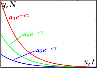
There is not just one solution but a whole class of solutions dependent on the intitial or boundary value, i.e. depending on how much radioactive material was present in the beginning.
| The generic form of a linear 1st order ODE is | $\frac{{\rm d}y}{{\rm d}x}+p(x)y=q(x)$. |
| The corresponding homogeneous equation is | $\frac{{\rm d}y}{{\rm d}x}+p(x)y=0$, |
| which can be separated: | $\frac{{\rm d}y}{y}=-p(x){\rm d}x$, |
| integrated: | $\ln{y}=-\int{p(x){\rm d}x}+c$, |
| and solved for $y$: | $y={\rm e}^{-\int{p(x){\rm d}x}+c}=A{\rm e}^{-\int{p(x){\rm d}x}}\qquad$(1), |
| where | $A:={\rm e}^c$. |
| Let the integral in the exponent | $I:=\int{p(x){\rm d}x}$ |
| and differentiate: | $\frac{{\rm d}I}{{\rm d}x}=p(x)\qquad$(2). |
| Substitute (2) into (1): | $y=A{\rm e}^{-I}$, which looks much friendlier! |
| Rearrange: | $y{\rm e}^I=A$ |
| and differentiate: | $\frac{{\rm d}}{{\rm d}x}y{\rm e}^I=\frac{{\rm d}A}{{\rm d}x}$. |
| Apply chain rule to LHS: | $\frac{\rm d}{{\rm d}x}y{\rm e}^I=\frac{{\rm d}y}{{\rm d}x}{\rm e}^I+y{\rm e}^I\frac{{\rm d}I}{{\rm d}x}$, |
| substitute (2) into it and simplify: | $=\frac{{\rm d}y}{{\rm d}x}{\rm e}^I+y{\rm e}^Ip(x)={\rm e}^I\color{red}{\left(\frac{{\rm d}y}{{\rm d}x}+yp(x)\right)}$. |
| The highlighted part happens to be the LHS of the ODE we started with, and we can substitute it into the last equation: | $\frac{\rm d}{{\rm d}x}y{\rm e}^I={\rm e}^I\left(\frac{{\rm d}y}{{\rm d}x}+yp(x)\right)=q(x){\rm e}^I$. |
| Integrate: | $y{\rm e}^I=\int{q(x){\rm e}^I{\rm d}x}+c$. That's it. |
Of course you don't need to do all this every time you need to solve a linear 1st order ODE.
| When you come across such an equation of the form | $\frac{{\rm d}y}{{\rm d}x}+p(x)y=q(x)$, |
| simply find the integrating factor | $I:=\int{p(x){\rm d}x}$ |
| and then evaluate | $y={\rm e}^{-I}\left(\int{q(x){\rm e}^I{\rm d}x}+c\right)$, |
where c is an integration constant that you may be able to fix if you have suitable physical boundary conditions.
If an ODE is neither separable nor linear, you can try if it fits one of a number of other patterns. A common pattern is the Bernoulli type, which is a 1st order ODE containing higher powers of the dependent variable but not of its derivatives.
| The general Bernoulli equation is | $\frac{{\rm d}y}{{\rm d}x}+p(x)y=q(x)y^n$. |
| Let | $z:=y^{1-n}$ |
| and differentiate: | $\frac{{\rm d}z}{{\rm d}x}=(1-n)y^{-n}\frac{{\rm d}y}{{\rm d}x}$ |
| (since | $\frac{{\rm d}z}{{\rm d}x}=\frac{{\rm d}z}{{\rm d}y}\cdot\frac{{\rm d}y}{{\rm d}x}=\frac{{\rm d}y}{{\rm d}x}\cdot\frac{{\rm d}}{{\rm d}y}y^{1-n}=\frac{{\rm d}y}{{\rm d}x}(1-n)y^{-n}\qquad$). |
| Multiply the original equation by $(1-n)y^{-n}$: | $(1-n)y^{-n}\frac{{\rm d}y}{{\rm d}x}+(1-n)y^{-n}p(x)y=(1-n)y^{-n}q(x)y^{n}$, |
| combine the $y$-terms: | $(1-n)y^{-n}\frac{{\rm d}y}{{\rm d}x}$ $+(1-n)$ $y^{1-n}$ $p(x)=(1-n)q(x)$. |
| and substitute $z$ and $z'$: | $\frac{{\rm d}z}{{\rm d}x}+(1-n)zp(x)=(1-n)q(x)$. |
This is a linear 1st order ODE and can be solved as described above. Solve for $z(x)$ and resubstitute to get $y(x)$. Don't forget the prefactor (1-$n$) in front of $p(x)$ and $q(x)$!
In the previous cases, $p(x)$ and $q(x)$ were funtions of the independent variable only. Here, we drop this assertion and write $p(x,y)$ and $q(x,y)$. Note, however, that these functions must not contain any differentials.
| A general homogeneous equation is | $p(x,y){\rm d}x+q(x,y){\rm d}y=0$. |
| We can rewrite this as | $\frac{{\rm d}y}{{\rm d}x}=-\frac{p(x,y)}{q(x,y)}$, which is more likely to be encountered anyway. |
| Defining $f(\frac{y}{x}):=-\frac{p(x,y)}{q(x,y)}$, we have | $\frac{{\rm d}y}{{\rm d}x}=f(\frac{y}{x})$. |
| Also define $v:=\frac{y}{x}$: | $\frac{{\rm d}y}{{\rm d}x}=f(v)$ and $y=vx$. |
| Differentiate (chain rule!): | $\frac{{\rm d}y}{{\rm d}x}=\frac{\rm d}{{\rm d}x}vx=x\frac{{\rm d}v}{{\rm d}x}+v$ |
| Solve for $\frac{{\rm d}v}{{\rm d}x}$: | $\frac{{\rm d}v}{{\rm d}x}=\frac{1}{x}\left(\frac{{\rm d}y}{{\rm d}x}-v\right)$ |
| and substitute: | $\frac{{\rm d}v}{{\rm d}x}=\frac{f(v)}{x}$, |
| which is separable: | $\frac{{\rm d}v}{f(v)}=\frac{{\rm d}x}{x}$. |
Solve for $v(x)$ and resubstitute.
These tools should be sufficient to solve the majority of ODE. Another type, linear ODE of any order with constant coefficients, will be treated later on. For now, let's find out how to fix boundary conditions.
At this point, you may want to try the first worksheet. Check your solutions when you've finished.