Fourier series are used to approximate non-periodic functions by a linear combination of periodic functions. In practice, more and more harmonics are added up until a shape sufficiently close to that of the original non-periodic function is obtained.
| series | formula | used for | |
|---|---|---|---|
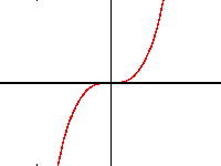
| Fourier sine series | $f(x)=\sum_{n=1}^{\infty}b_n\sin{(\frac{n\pi x}{l})}$ | odd functions: $f(-x)=-f(x)$ |  |
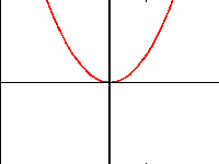
| Fourier cosine series | $f(x)=\sum_{n=1}^{\infty}b_n\cos{(\frac{n\pi x}{l})}$ | even functions: $f(-x)=f(x)$ |  |
| complex Fourier series | $f(x)=\sum_{n=1}^{\infty}b_n{\rm e}^{{\rm i}\frac{n\pi x}{l}}$ | functions with other or no symmetry | |
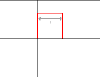
| Assume we have a non-periodic function, | $f(x)=\begin{cases}1&(\text{for}\quad 0\lt x\lt\pi)\\0&(\text{otherwise})\end{cases}$: |  |
. |
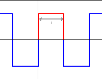
| We can think of this as a section of an odd periodic function, | $g(x)=\begin{cases}1&(\text{for}\quad 2m\pi\lt x\lt(2m+1)\pi)\\-1&(\text{otherwise})\end{cases}$: |  |
. |
Within the limits in which $f(x)$ is defined, $f(x)=g(x)$, so it doesn't matter what we add outside the limits.
| The coefficients of the sine series, | $f(x)=\sum_{n=1}^{\infty}b_n\sin{\frac{n\pi x}{l}}$, | |
| are found by solving the integral | $b_n=\frac{2}{l}\int_0^lf(x)\sin{\frac{n\pi x}{l}}{\rm d}x$ , | |
| where $l$ is half the period of the fundamental ($n=1$) oscillation. | ||
| Insert $f(x)$ and $l$: | $=\frac{2}{\pi}\int_0^{\pi}1\sin{\frac{n\pi x}{\pi}{\rm d}x}=\frac{2}{\pi}\int_0^{\pi}\sin{nx}{\rm d}x$, | |
| integrate: | $=\frac{2}{n\pi}[\cos{nx}]_0^{\pi}$, | |
| and substitute the limits: | $=\begin{cases}\frac{4}{n\pi}&(\text{for $n$ odd})\\0&(\text{for $n$ even})\end{cases}$. | |
| Hence, $f(x)$ can be expressed as: | $$f(x)=\frac{4}{\pi}\sum_{{\rm odd} n=0}^{\infty}\frac{\sin{nx}}{n}$$ | |
The image on the right shows the first five odd terms ($n=1,3,5,7,9$) and how they gradually build up the shape of the top-hat function. The Fourier coefficients of the even terms are zero as shown above; therefore they aren't shown. The individual Fourier terms are plotted in green and their sum in blue. Note that the amplitude of each term is smaller than that of its predecessor, i.e. the corrections are getting smaller each time.
We can now finish solving Laplace's equation.