Fourier transformation 3 - transforming in practice


This page contains a number of examples which resemble time-domain data obtained with a Fourier-transform spectrometer such as widely used for nuclear magnetic resonance (NMR) and infrared (IR) spectroscopy. These signals are typically exponential decays with several superimposed oscillations. The decay transforms into the line width, while the oscillations show up as line positions in the Fourier transform, i.e. the spectrum. If you have gnuplot or MathCAD or the like, you can try this at home; this worksheet gives instructions.
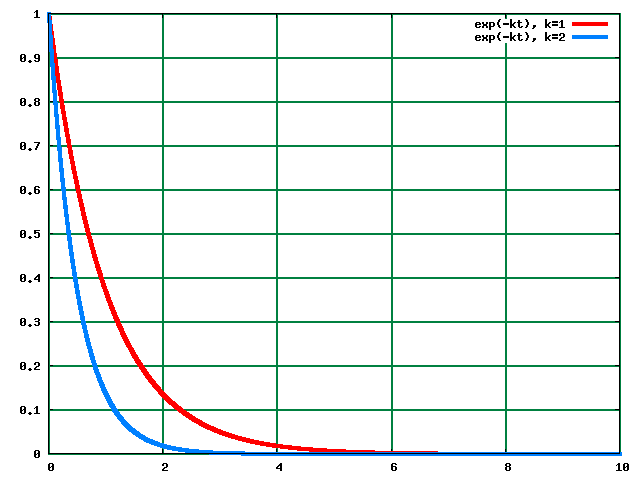
| A real-only single-exponential decay | $f(t)= {\rm e}^{-kt}(+{\rm i}0)$ |
| transforms as | $$F(\omega)=\frac{1}{2\pi}\int_{-\infty}^{+\infty}{\rm e}^{-kt}{\rm e}^{-{\rm i}\omega t}{\rm d}t\qquad.$$ |
If we let the time axis begin at zero and, from a point $a$ onwards, the signal is practically indistinguishable from zero,
| then the limits become | $$=\frac{1}{2\pi}\int_0^a{\rm e}^{-(k+{\rm i}\omega)t}{\rm d}t\qquad.$$ |
| Integrate: | $=\frac{1}{2\pi}\left[-\frac{1}{k+{\rm i}\omega}{\rm e}^{-(k+{\rm i}\omega)t}\right]_0^a\qquad,$ |
| substitute limits: | $=\frac{1}{2\pi}(0+\frac{1}{k+{\rm i}\omega})$ |
| (the first term is zero by definition of $a$ as the cut-off value). | |
| Tidy up: | $=\frac{1}{2\pi k+{\rm i}2\pi\omega}\qquad.$ |
| To see what the real and imaginary parts of the solution are, it is better to get rid of the complex unit in the denominator. This can be done by multiplying both numerator and denominator by the conjugate of the denominator: | |
| $=\frac{2\pi k-{\rm i}2\pi\omega}{4\pi^2k^2+4\pi^2\omega^2}\qquad.$ | |
| Tidy up again: | $=\frac{k-{\rm i}\omega}{2\pi(k^2+\omega^2)}\qquad.$ |
 Click image to Fourier transform. (Alternatively, view Fourier transform here.)
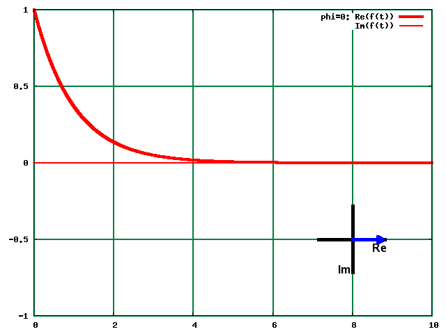
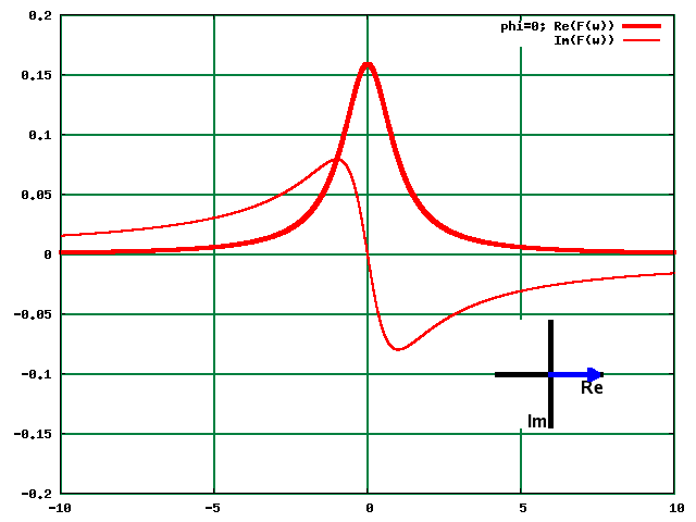
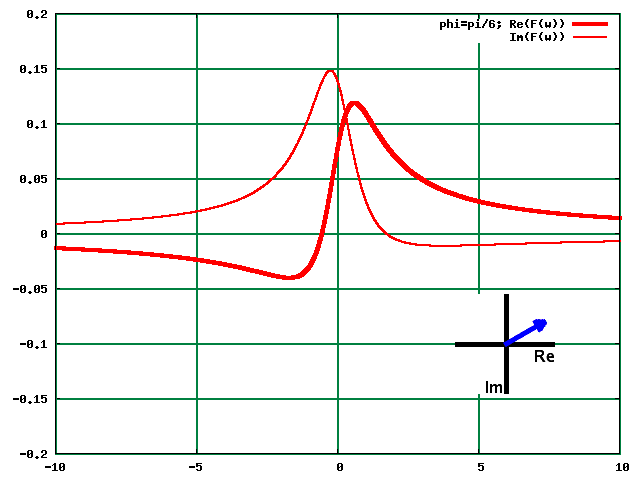
In the example above, the input function was real-only. In general, there will be a phase factor which determines how the intensity is distributed between the real and imaginary parts.
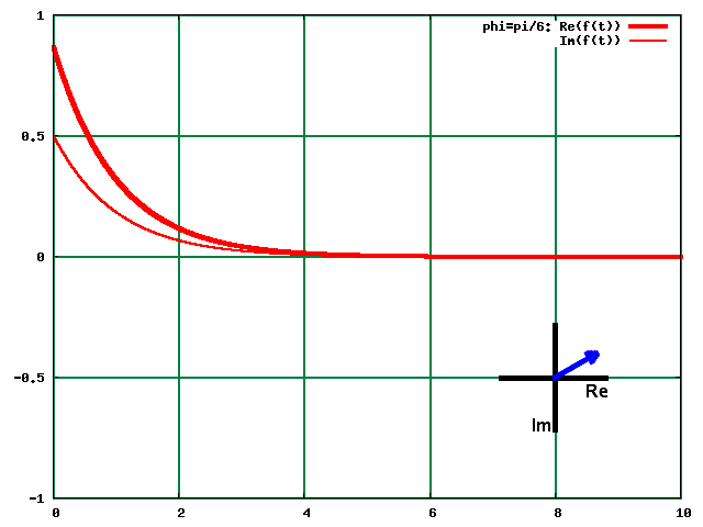
| Decay function with phase factor: | $f(t)= {\rm e}^{-kt}{\rm e}^{{\rm i}\phi}\qquad,$ |
| which is the same as | $f(t)= {\rm e}^{-kt}(\cos\phi+{\rm i}\sin\phi)\qquad,$ |
| i.e. the real and imaginary parts are modulated by a cosine and sine wave, respectively. | |
| The Fourier transform is: | $$F(\omega)=\frac{1}{2\pi}\int_0^a{\rm e}^{-kt}{\rm e}^{{\rm i}\phi}{\rm e}^{-{\rm i}\omega t}{\rm d}t\qquad.$$ |
| The phase factor doesn't depend on $t$. So, | $$=\frac{{\rm e}^{{\rm i}\phi}}{2\pi}\int_0^a{\rm e}^{-(k+{\rm i}\omega)t}{\rm d}t\qquad,$$ |
| which contains the same integral as above: | $={\rm e}^{{\rm i}\phi}\frac{k-{\rm i}\omega}{2\pi(k^2+\omega^2)}\qquad.$ |
This results in the following time-domain signals and spectra (click images to transform):
 Click image to Fourier transform. (Alternatively, view Fourier transform here.)
 Click image to Fourier transform. (Alternatively, view Fourier transform here.)
 Click image to Fourier transform. (Alternatively, view Fourier transform here.)
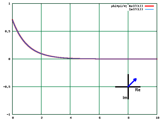
At $\frac{\pi}{4}$, real and imaginary part of the input function are identical. In the corresponding spectrum, the real and imaginary lines are mirror images of each other. The mirror is the parallel of the $y$ axis at the position of the line (here $x=0$).
 Click image to Fourier transform. (Alternatively, view Fourier transform here.)
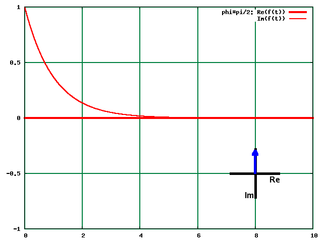
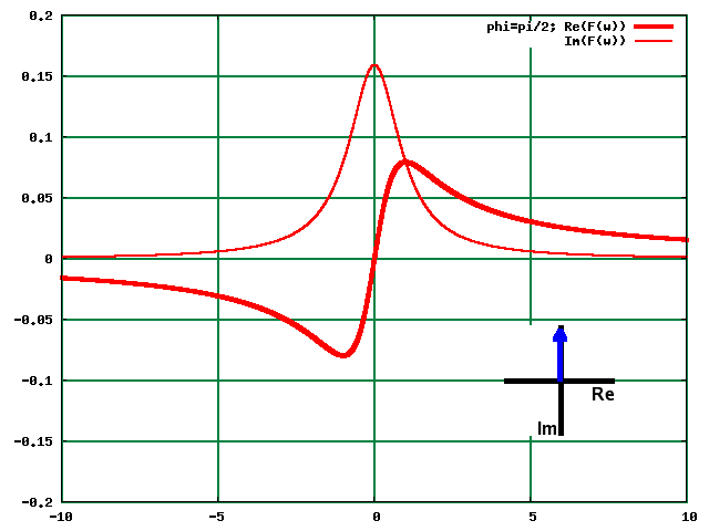
At $\frac{\pi}{2}$, the real and imaginary parts are swapped w.r.t. the original function. In the spectrum, the two components swap also. Note that the real part now is a mirror image of the original imaginary part (because Im is always behind Re by $\frac{\pi}{2}$).
 Click image to Fourier transform. (Alternatively, view Fourier transform here.)
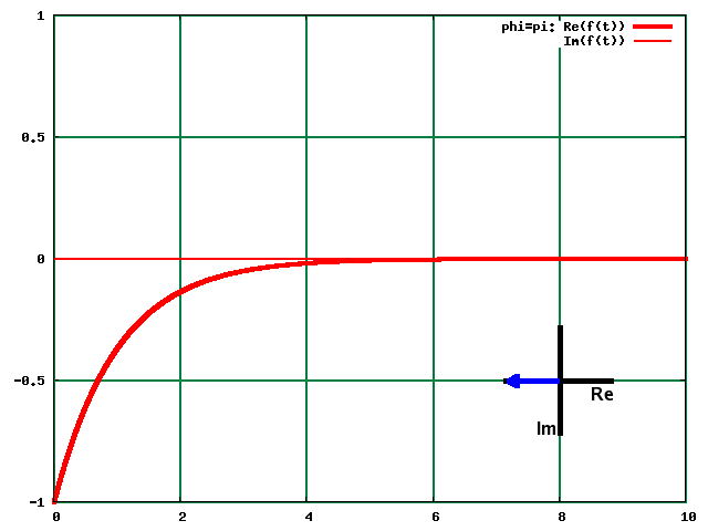
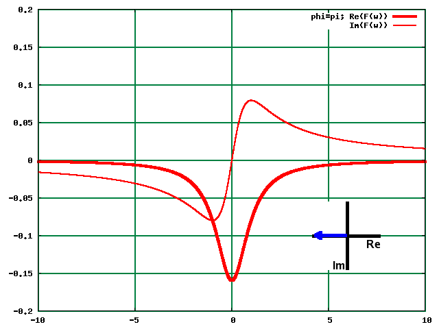
At $\pi$, the real part is inverted; hence the spectrum is also inverted.
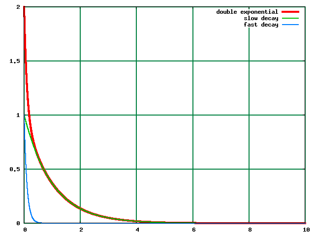
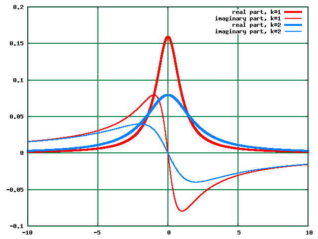
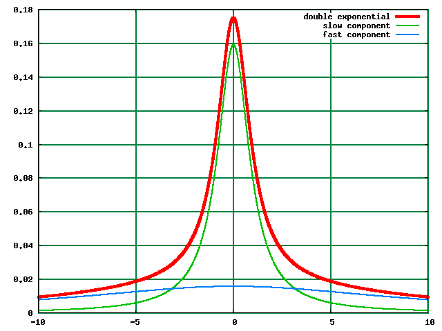
| The sum of two decays: | $f(t)= {\rm e}^{-k_1t}+{\rm e}^{-k_2t}$ |
| transforms as | $$=F(\omega)=\frac{1}{2\pi}\int_0^a({\rm e}^{-k_1t}+{\rm e}^{-k_2t}){\rm e}^{-{\rm i}\omega t}{\rm d}t\qquad.$$ |
| That integral can be split: | $$=\frac{1}{2\pi}\int_0^a{\rm e}^{-(k_1+{\rm i}\omega)t}{\rm d}t+\frac{1}{2\pi}\int_0^a{\rm e}^{-(k_2-{\rm i}\omega)t}{\rm d}t$$ |
| into two of the usual form. Thus, | $=\frac{k_1-{\rm i}\omega}{2\pi(k_1^2+\omega^2)}+\frac{k_2-{\rm i}\omega}{2\pi(k_2^2+\omega^2)}\qquad.$ |
 Click image to Fourier transform. (Alternatively, view Fourier transform here.)
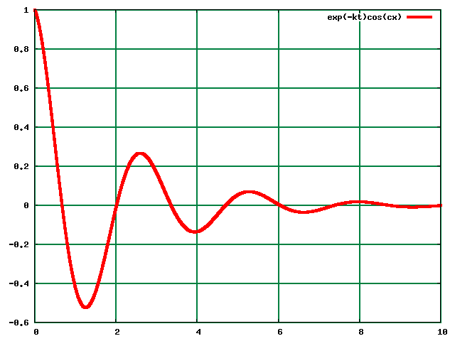
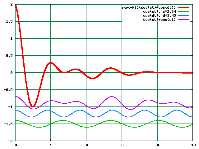
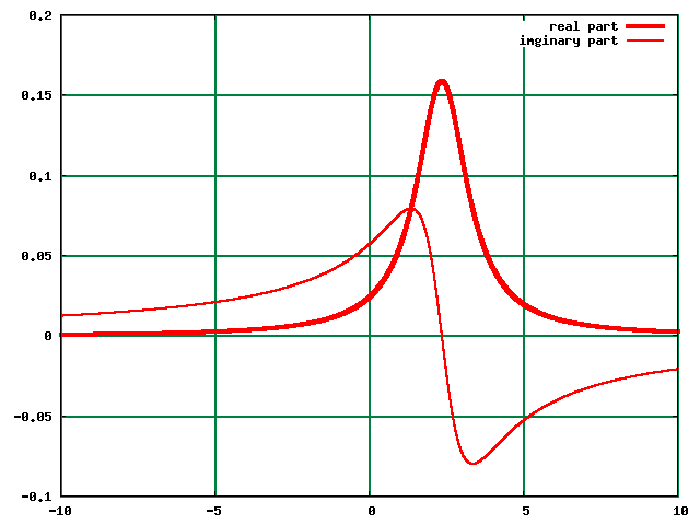
An oscillation is best described as a complex exponential. A damped oscillation is an exponential decay (as before) with an oscillation superimposed, i.e. multiplied to it.
| So, the input function is: | $f(t)= {\rm e}^{-kt}{\rm e}^{{\rm i}ct}\qquad,$ |
| which transforms as: | $$="F(\omega)=\frac{1}{2\pi}\int_0^a{\rm e}^{-kt}{\rm e}^{{\rm i}ct}{\rm e}^{-{\rm i}\omega t}{\rm d}t\qquad.$$ |
| Integrate: | $=\frac{1}{2\pi}\left[-\frac{{\rm e}^{-(k+{\rm i}(\omega-c))t}}{k+{\rm i}(\omega-c)}\right]_0^a\qquad,$ |
| substitute limits: | $=\frac{1}{2\pi}\frac{1}{k+{\rm i}(\omega-c)}\qquad,$ |
| and tidy up | $=\frac{1}{2\pi}\frac{k-{\rm i}(\omega-c)}{k^2+(\omega-c)^2}\qquad.$ |
 Click image to Fourier transform. (Alternatively, view Fourier transform here.)
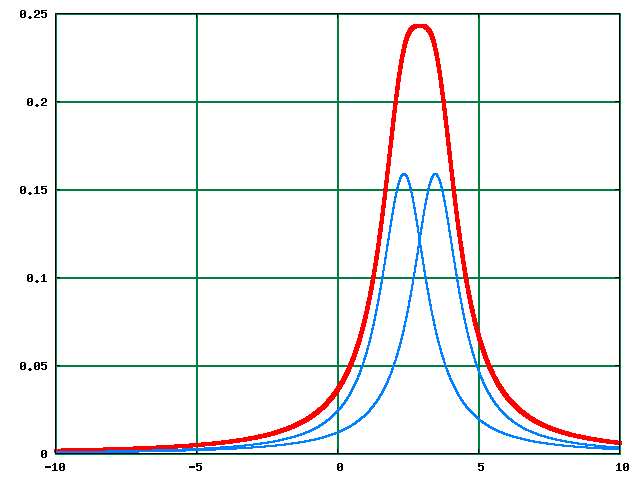
In a system with two different energy transitions, photons of two different frequencies will be absorbed. Thus we have an exponential decay with two superimposed frequencies: $f(t)= {\rm e}^{-kt}\left({\rm e}^{{\rm i}c_1t}+{\rm e}^{{\rm i}c_2t}\right)\qquad$.
According to the addition theorem, these give rise to two separate lines, each shifted by their frequencies $c_1$ and $c_2$, respectively.
 Click image to Fourier transform. (Alternatively, view Fourier transform here.)
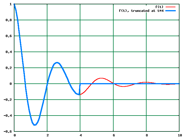
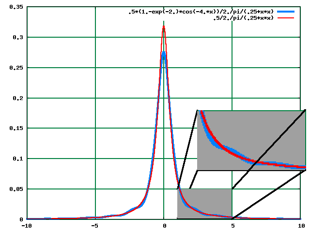
Experimental data sets cannot continue forever. If a data set is truncated before all oscillations have petered out, the spectroscopist's pet artifact, the dreaded Fourier wiggles, are created.
So far, we have assumed that we can terminate the integration at some value a at which the signal becomes indiscernible from zero. Here's what happens if the input function drops to zero immediately, i.e. the data set ends prematurely.
| Multiply the usual decay by a step function: | $f(t)= {\rm e}^{-kt}z(t)\qquad,$ |
| where | $z(t):=\begin{cases}1&(x\leq b)\\0&(x >b)\end{cases}\qquad,$ |
| where $f(t)$ is still discernible from zero at $t=b$. | |
| The Fourier transform is: | $$F(\omega)=\frac{1}{2\pi}\int_0^a{\rm e}^{-kt}z(t){\rm e}^{-{\rm i}\omega t}{\rm d}t\qquad,$$ |
| but $z(t)$ forces $f(t)=0$ for $t\gt b$: | $$=\frac{1}{2\pi}\int_0^b{\rm e}^{-(k+{\rm i}\omega)t}{\rm d}t\qquad.$$ |
| Integrate: | $$=\frac{1}{2\pi}\left[-\frac{{\rm e}^{-(k+{\rm i}\omega)t}}{k+{\rm i}\omega}\right]_0^b$$ |
| and substitute limits: | $=\frac{1}{2\pi}\left(-\frac{1}{k+{\rm i}\omega}{\rm e}^{-(k+{\rm i}\omega)b}+\frac{1}{k+{\rm i}\omega}\right)$ |
| because this time, at $t=b$, $f(t)$ hasn't decayed completely yet. | |
| Tidy up: | $=\frac{k-{\rm i}\omega}{2\pi(k^2+\omega^2)}\left(1-{\rm e}^{-(k+{\rm i}\omega)b}\right)\qquad.$ |
 Click image to Fourier transform. (Alternatively, view Fourier transform here.)
That concludes the section on Fourier transforms. Here's the associated worksheet and its solutions.
There's also a toolbox sheet to help you revise.