Introduction to Fourier transforms :: Advanced Techniques

Complex exponentials are periodic functions

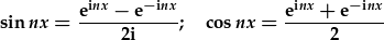
Real sines and cosines can be expressed as complex exponentials:
$\sin{nx}=\frac{\ur{e}^{\ur{i}nx}-\ur{e}^{-\ur{i}nx}}{2\ur{i}};\quad\cos{nx}=\frac{\ur{e}^{\ur{i}nx}+\ur{e}^{-\ur{i}nx}}{2}$
Many physical processes are periodic and can be treated as superpositions of sine or cosine functions. In addition, we have seen that many functions, even non-periodic ones, can be expanded into Fourier series, i.e. series of harmonic sine or cosine (or, more general, complex exponential) functions.

Fourier coefficients

In the pure real sine series,	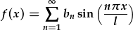$f(x)=\sum_{n=1}^{\infty}b_n\sin{(\frac{n\pi x}{l})}$ ,
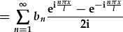
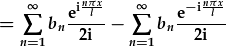
substitute the sine by complex exponentials:	$=\sum_{n=1}^{\infty}b_n\frac{\ur{e}^{\ur{i}\frac{n\pi x}{l}}-\ur{e}^{-\ur{i}\frac{n\pi x}{l}}}{2\ur{i}}$
and split the sum:	$=\sum_{n=1}^{\infty}b_n\frac{\ur{e}^{\ur{i}\frac{n\pi x}{l}}}{2\ur{i}}-\sum_{n=1}^{\infty}b_n\frac{\ur{e}^{-\ur{i}\frac{n\pi x}{l}}}{2\ur{i}}$ .
The sum of -n from 1 to infinity is the same as the sum of +n from -infinity to -1.
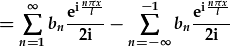So, we can count the second sum backwards:	$=\sum_{n=1}^{\infty}b_n\frac{\ur{e}^{\ur{i}\frac{n\pi x}{l}}}{2\ur{i}}-\sum_{n=-\infty}^{-1}b_n\frac{\ur{e}^{\ur{i}\frac{n\pi x}{l}}}{2\ur{i}}$ .
Now that both sums are the same, we can put them together:	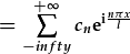$=\sum_{-infty}^{+\infty}c_n\ur{e}^{\ur{i}\frac{n\pi x}{l}}$ ,
where	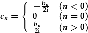$c_n={\begin{array}{ll}-\frac{b_n}{2\ur{i}}&(n<0)\\0&(n=0)\\\frac{b_n}{2\ur{i}}&(n>0)\end{array}$

Note that for the pure sine series, c₀=0, but in general (cosine or mixed series included) this will not be the case. In general,

the c_n are found by	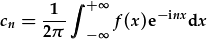$c_n=\frac{1}{2\pi}\int_{-\infty}^{+\infty}f(x)\ur{e}^{-\ur{i}nx}\ur{d}x$
to expand	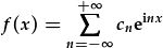$f(x)=\sum_{n=-\infty}^{+\infty}c_n\ur{e}^{\ur{i}nx}$ .

Discrete Fourier series and continuous Fourier transforms

So, we need to solve an integral to find the coefficients in the Fourier series. The exponents in the series and in the integral are the same apart from the sign. This symmetry can be exploited to move from a discrete Fourier series to a continuous Fourier transform:

discrete	->	continuous
index variable n	->	continuous variable q
Fourier coefficients c_n	->	Fourier transform g(q)
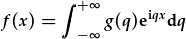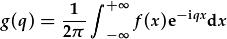$f(x)=\sum_{n=-\infty}^{+\infty}c_n\ur{e}^{\ur{i}nx}$	->	$f(x)=\int_{-\infty}^{+\infty}g(q)\ur{e}^{\ur{i}qx}\ur{d}q$
$c_n=\frac{1}{2\pi}\int_{-\infty}^{+\infty}f(x)\ur{e}^{-\ur{i}nx}\ur{d}x$	->	$g(q)=\frac{1}{2\pi}\int_{-\infty}^{+\infty}f(x)\ur{e}^{-\ur{i}qx}\ur{d}x$

The set of coefficients c_n depending on a discrete index varable n is replaced by a continuous function g(q) depending on a continuous variable q.
g(q) is the Fourier transform of f(x); f(x) is the inverse Fourier transform of g(q). Note the symmetry!

Fourier pairs in physics

Because of the symmetry of Fourier transform and inverse Fourier transform, many physical properties come in Fourier pairs: measure one and get the complementary one by Fourier transformation. This is an extremely useful technique and is very widespread in experimental physics. The two most common examples are spectroscopic and scattering techniques:

Spectrosopy: Time and frequency
Transitions between energy levels (e.g. different molecular vibration states or excited electron states in semiconductors etc.) require a certain amount of energy, which is supplied by a photon of the corresponding frequency. However, it is often easier to irradiate the sample with a white source (i.e. a light source which contains all frequencies in the relevant band) and measure a response of the sample as function of time. This saves the effort of monochromatising the incoming radiation and is also much faster. The signal f(t) measured as a function of time t is then Fourier transformed to reveal the frequency spectrum $g(\nu)$ , of the system under study.
Scattering: Space and reciprocal space
When photons are diffracted by a lattice plane of a crystal, positive interference as a result of scattering with different atoms in symmetrically equivalent locations produces maxima of scattered intensity at certain angles with respect to the incoming beam. Such Bragg peaks appear at large angles if the correlated scatterers are close to each other, and at small angles if they are far apart: diffraction maps reciprocal space. In order to obtain information on the real space, i.e. the actual positions of atoms, a Fourier transformation of the scattering pattern is required. The Fourier transform g(r) contains the same information as the original pattern f(q); therefore it is customary to interpret diffraction patterns in reciprocal space. However, it is easier to work out the coordination numbers (number of direct neighbours) of atoms in real space, in which case the data are Fourier transformed.

When computing Fourier transforms, symmetries can often be used to improve efficiency.