Mathcad's FT functions


The best way to get used to thinking Fourier is to keep on practising. Think of a number of increasingly complicated functions, add noise and truncate to taste, then predict what the Fourier transform is going to look like. You can use Mathcad to check your Fourier instinct.
To add noise, you can use a random number generator. Mathcad's rnd(c) function produces
noise in the range from 0 to c. Because noise can be positive or negative, subtract half of the noise
amplitude c from each data point:
noise(x) = rnd(c) - c/2.
This uses a different random number for each value of x.
For truncating, Mathcad has the Heaviside step function, Phi(d). It evaluates as zero if d is
negative and as one otherwise. To truncate an input function, we want to set all values above
a certain cutoff x value to zero. Therefore, we need to invert the argument of the Heaviside
function (to make positive values vanish instead of negative ones) and then shift the cutoff to the
x value where we want it:
trunc(x) = Phi(d-x)
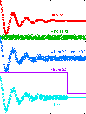
Now consider that you want to add the noise to your input function, then set all values above
the cutoff to zero by multiplying with the Heaviside function. Therefore, if func(x) is
the function you want to transform, then the "massaged" input function is
f(x) = ( func(x) + rnd(c) - c/2 ) • Phi(d-x)
The FFT routine is meant to work with discrete data sets. Therefore, the Mathcad Fourier routines expect
a vector rather than a continuous function as input. Define your x range as a
range variable
e.g. x := 0..1023
and define f as a discrete vector fx rather than continuous function f(x).
Remember that the FFT algorithm requires a power-of-two size input vector.
Mathcad has eight different Fourier functions, four pairs of transform and inverse transform. The prefix
i indicates the inverse transform. Functions with the prefix c are the most general versions
for complex input data; those lacking the c are for real-only input data. The lower-case
and capitalised versions differ in the normalisation convention.
![[c]fft(q)=\frac{1}{\sqrt{N}}\int_{x_0}^{x_N}f(x)e^{+iqx}dx\\ i[c]fft(x)=\frac{1}{\sqrt{N}}\int_{q_0}^{q_N}g(q)e^{-iqx}dq\\ [C]FFT(q)=\frac{1}{N}\int_{x_0}^{x_N}f(x)e^{-iqx}dx\\ I[C]FFT(x)=\int_{q_0}^{q_N}g(q)e^{+iqx}dq](ft_mathcad_2.png)
When transforming back and forth, it is important to use Fourier and inverse Fourier transformation from the
same pair, e.g cfft(q) and icfft(x). The lower-case functions have the advantage that
the normalisation factor is the same either way, which is usually appropriate in physics, where intensity
(i.e. the integral) is preserved. The use of the real-only versions save some memory where
appropriate by exploiting symmetry, but on today's computers that is hardly
an issue with one-dimensional data sets. So, generally, cfft(q) and icfft(x) are the best
choice.
As an exercise, write a Mathcad script such as this. To check, compare with this example script. Change the parameters, input function, and FFT routine in the yellow fields.