
The Schrödinger equation, $\hat{H}\psi=E\psi$, gives us two handles to refine a problem to make it more realistic: the Hamiltonian and the wave function. The energy eigenvalues are just scalar values that respond to changes we make to the other terms. The two approaches are compared below.
In both cases (and more generally, too), the energy eigenvalues are found using
$$E=\int_{-\infty}^{\infty}\psi^*\hat{H}\psi{\rm d}x\qquad.$$
This prescribes a method of calculation which involves three steps:
The recipe must be followed in this particular order as operators and their operands in general do not commute, i.e. the result is different depending on the order the terms are applied.
Two (or more) wave functions are mixed by linear combination. The coefficients $c_1,c_2$ determine the weight each of them is given. The optimum coefficients are found by searching for minima in the potential landscape spanned by $c_1$ and $c_2$.
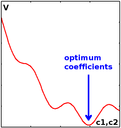
The energy minima are found by finding the differentials $$\frac{\partial E}{\partial c_1}=\frac{\partial E}{\partial c_2}=0$$ and setting them to zero.
Given that $$\begin{eqnarray*}E&=&\int\psi^*\hat{H}\psi{\rm d}x\\&=&\int(c_1\psi_1^*+c_2\psi_2^*)\hat{H}(c_1\psi_1+c_2\psi_2){\rm d}x\quad,\end{eqnarray*}$$ we see that the energy eigenvalue has separate contributions coming from $\psi_1$ or $\psi_2$ only: $$=c_1^2\int\psi_1^*\hat{H}\psi_1{\rm d}x+c_2^2\int\psi_2^*\hat{H}\psi_2{\rm d}x\,+\cdots$$ and a cross term known as the overlap integral: $$\cdots+\,c_1c_2\left(\int\psi_1^*\hat{H}\psi_2{\rm d}x+\int\psi_2^*\hat{H}\psi_1{\rm d}x\right)\quad.$$
In molecular physics, the overlap integral causes the difference in energy between bonding and anti-bonding molecular states.
The unperturbed Hamiltonian of a known system is modified by adding a perturbation with a variable control parameter $\lambda$, which governs the extent to which the system is perturbed.
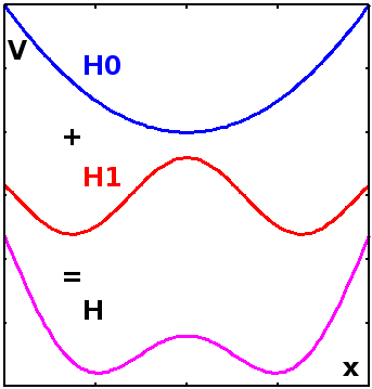
The perturbation can affect the potential, the kinetic energy part of the Hamiltonian, or both. As an example, consider a double well potential created by superimposing a periodic potential on a parabolic one. This might apply e.g. to a defect in a crystalline lattice.
The Schrödinger equation for the perturbed system is $$\hat{H}\psi_n=E_n\psi_n\quad,$$ that for the unperturbed (known) system is $$\hat{H}_0\psi_n^0=E_n^0\psi_n^0\quad.$$ The index $n$ just serves to identify a particular wave function (e.g. one which uses the same quantum number both for the perturbed and the unperturbed variant).
We'll leave the fine detail of the variation technique to the fourth-year module, but will derive here a recipe (for the impatient: it's highlighted at the bottom!) by which we can determine the energy correction due to a perturbation acting on a known system (i.e. one whose Hamiltonian, wave functions and eigenvalues we know already).
The Schrödinger equation of the perturbed system contains the perturbing Hamiltonian (known) and the perturbed wave functions and eigenvalues (as yet unknown): $$\hat{H}\psi_n=(\hat{H}_0+\lambda\hat{H}_1)\psi_n=E_n\psi_n\quad.$$
Since both wave functions and eigenvalues are unknown, they are expanded into Taylor series as an approximation (leaving out the index $n$ for clarity here):
$$\psi=\psi|_{\lambda=0}+\lambda\left.\frac{\partial\psi}{\partial\lambda}\right|_{\lambda=0}+\frac{\lambda^2}{2!}\left.\frac{\partial^2\psi}{\partial\lambda^2}\right|_{\lambda=0}+\frac{\lambda^3}{3!}\left.\frac{\partial^3\psi}{\partial\lambda^3}\right|_{\lambda=0}+\cdots\quad,$$
and
$$E=E|_{\lambda=0}+\lambda\left.\frac{\partial E}{\partial\lambda}\right|_{\lambda=0}+\frac{\lambda^2}{2!}\left.\frac{\partial^2E}{\partial\lambda^2}\right|_{\lambda=0}+\frac{\lambda^3}{3!}\left.\frac{\partial^3E}{\partial\lambda^3}\right|_{\lambda=0}+\cdots\quad.$$
Here, each term is a progressively smaller correction (i.e. the series converges to the true value of $\psi$ or $E$, respectively). To achieve this, they are weighted with prefactors in progressive powers of $\lambda$ and progressive inverse factorials -- the prefactors are diminishing very rapidly given that the control parameter $\lambda$ ranges from zero to one. The differentials take into account how $\psi$ and $E$ respond to changes in $\lambda$, i.e. the severity of the perturbation. The notation $\left.\right|_{\lambda=0}$ indicates that all differentials are evaluated in the limit of very small $\lambda$.
We can write the two series as sums: $$\psi=\sum_{i=0}^{\infty}\frac{\lambda^i}{i!}\left.\frac{\partial^i\psi}{\partial\lambda^i}\right|_{\lambda=0} \quad\textrm{and}\quad E=\sum_{i=0}^{\infty}\frac{\lambda^i}{i!}\left.\frac{\partial^iE}{\partial\lambda^i}\right|_{\lambda=0}\quad.$$ For ease of notation, we can bundle up the differentials and factorials into abbreviated symbols: $$\psi^{(i)}:=\frac{1}{i!}\left.\frac{\partial^i\psi}{\partial\lambda^i}\right|_{\lambda=0} \quad\textrm{and}\quad E^{(i)}:=\frac{1}{i!}\left.\frac{\partial^iE}{\partial\lambda^i}\right|_{\lambda=0}\quad.$$ Then $\psi^{(0)}$ and $E^{(0)}$ are the unperturbed wave functions and eigenvalues, while $\psi^{(i)}$ and $E^{(i)}$ are the changes to the wave functions and energy eigenvalues due to the perturbation, evaluated to the $i$-th order of perturbation theory. Using this, the two sums can be written as $$\psi=\sum_{i=0}^{\infty}\lambda^i\psi^{(i)} \quad\textrm{and}\quad E=\sum_{i=0}^{\infty}\lambda^iE^{(i)}\quad.$$
With the series expansions, the Schrödinger equation $\hat{H}\psi=E\psi$ becomes
$$(\hat{H}_0+\lambda\hat{H}_1)(\psi^{(0)}+\lambda\psi^{(1)}+\lambda^2\psi^{(2)}+\cdots)\\ =(E^{(0)}+\lambda E^{(1)}+\lambda^2E^{(2)}+\cdots)(\psi^{(0)}+\lambda\psi^{(1)}+\lambda^2\psi^{(2)}+\cdots)\quad.$$
By factoring out, we can split this into terms of different order in λ:
$$\color{red}{\hat{H}_0\psi^{(0)}}+\color{blue}{\lambda(\hat{H}_1\psi^{(0)}+\hat{H}_0\psi^{(1)})}+\lambda^2(\hat{H}_1\psi^{(1)}+\hat{H}_0\psi^{(2)})+\cdots\\ =\color{red}{E^{(0)}\psi^{(0)}}+\color{blue}{\lambda(E^{(0)}\psi^{(1)}+E^{(1)}\psi^{(0)})}+\lambda^2(E^{(0)}\psi^{(2)}+E^{(1)}\psi^{(1)}+E^{(2)}\psi^{(0)})+\cdots$$
The zeroth-order term corresponds to the unperturbed system, and we can use the first-order term to derive the energy corrections, $E^{(0)}$. The equation can be split into separate equations for each order, which can be solved independently.
Concentrating on the 1st-order equation, $$\bbox[lightblue]{\hat{H}_1\psi^{(0)}}+\bbox[lightgreen]{\hat{H}_0\psi^{(1)}}=E^{(0)}\psi^{(1)}+E^{(1)}\psi^{(0)}\quad,$$ we see that the LHS is the sum of the perturbation applied to the original wave function and the original Hamiltonian applied to the (unknown) 1st-order correction to the wave function.
Generally, as explained at the top of this page, we can find energy eigenvalues by sandwiching the Hamiltonian between the wave function and its complex conjugate and integrating over all space: $E=\int_{-\infty}^{\infty}\psi^*\hat{H}\psi{\rm d}x$. We can bring the LHS terms in that shape by multiplying from the left with $\psi_m^{(0)\ast}$ and integrating:
$$\int\psi_m^{(0)*}\hat{H}_1\psi_n^{(0)}{\rm d}x+\int\psi_m^{(0)*}\hat{H}_0\psi_n^{(1)}{\rm d}x=\int\psi_m^{(0)*}E_n^{(0)}\psi_n^{(1)}{\rm d}x+\int\psi_m^{(0)*}E_n^{(1)}\psi_n^{(0)}{\rm d}x\quad.$$
Here the index $n$ reappears, because the wave function we multiply the equation with needn't be the same as the one that's already there -- they could be ones with different values of a quantum number. To distinguish them, we use $m$ and $n$ as indices.
On the RHS, the energies are just scalars and can be taken outside the integrals:
$$\int\psi_m^{(0)*}\hat{H}_1\psi_n^{(0)}{\rm d}x+\bbox[pink]{\int\psi_m^{(0)*}\hat{H}_0\psi_n^{(1)}{\rm d}x}=E_n^{(0)}\int\psi_m^{(0)*}\psi_n^{(1)}{\rm d}x+E_n^{(1)}\int\psi_m^{(0)*}\psi_n^{(0)}{\rm d}x\quad.$$
Since the energy eigenvalue must be a real number rather than a complex one, the result of $$E=\int_{-\infty}^{\infty}\psi^*\hat{H}\psi{\rm d}x$$ must be real. This is the case if the imaginary parts of $\psi^{\ast}$ and $\hat{H}\psi$ just cancel out, i.e. $$\int\psi^*\hat{H}\psi{\rm d}x\stackrel{!}{=}\int\psi(\hat{H}\psi)^*{\rm d}x\quad.$$ Any operator that meets this criterion is described as an Hermitian operator, after mathematician Charles Hermite. All Hamiltonians in quantum mechanics are Hermitian, but the mathematical concept is not limited to quantum mechanics.
It is also useful to consider that $xy^{\ast}=(x^{\ast}y)^{\ast}$, as we can see by factorising the two complex numbers $x=a+{\rm i}b$ and $y=c+{\rm i}d$: $$xy^{\ast}=(a+{\rm i}b)(c-{\rm i}d)\\=ac-{\rm i}ad+{\rm i}bc+bd\\=(ac+bd)+{\rm i}(bc-ad)$$ and $$(x^{\ast}y)^{\ast}=\left((a-{\rm i}b)(c+{\rm i}d)\right)^{\ast}\\=(ac+bd)+{\rm i}(bc-ad)$$ Thus $xy^{\ast}=(x^{\ast}y)^{\ast}$.
The second term on the left needs some further attention. Because the Hamilton operator is Hermitian (see box), we can swap the two wave functions: $$\bbox[pink]{\int\psi_m^{(0)*}\hat{H}_0\psi_n^{(1)}{\rm d}x}=\int\psi_n^{(1)}(\hat{H}_0\psi_m^{(0)})^*{\rm d}x$$ Using $xy^{\ast}=(x^{\ast}y)^{\ast}$ (see box), we have $$=\int(\psi_n^{(1)*}\hat{H}_0\psi_m^{(0)})^*{\rm d}x\quad,$$ and the integral doesn't interfere with the complex conjugate: $$=\left[\int\psi_n^{(1)*}\hat{H}_0\psi_m^{(0)}{\rm d}x\right]^*\quad.$$ Now, $H_0\psi_m^{(0)}$ is just the LHS of the unperturbed Schrödinger equation for state $m$, and we can replace it with the corresponding RHS: $$=\left[\int\psi_n^{(1)*}E_m^{(0)}\psi_m^{(0)}{\rm d}x\right]^*\quad,$$ and since the eigenvalue is constant and real, it can be taken out of the integral and lose its complex-conjugate asterisk: $$=E_m^{(0)}\left[\int\psi_n^{(1)*}\psi_m^{(0)}{\rm d}x\right]^*\quad.$$ Finally, we just need to undo the double complex conjugate: $$=E_m^{(0)}\int\psi_m^{(0)*}\psi_n^{(1)}{\rm d}x\quad.$$
With the second term of the perturbed Schrödinger equation now simplified, we have:
$$\int\psi_m^{(0)*}\hat{H}_1\psi_n^{(0)}{\rm d}x+\bbox[pink]{E_m^{(0)}\int\psi_m^{(0)*}\psi_n^{(1)}{\rm d}x}=E_n^{(0)}\int\psi_m^{(0)*}\psi_n^{(1)}{\rm d}x+E_n^{(1)}\int\psi_m^{(0)*}\psi_n^{(0)}{\rm d}x\quad.$$
Note that the second and third integral are the same, so we can combine the two terms on the LHS and put the other two on the right:
$$(E_m^{(0)}-E_n^{(0)})\int\psi_m^{(0)*}\psi_n^{(1)}{\rm d}x=E_n^{(1)}\int\psi_m^{(0)*}\psi_n^{(0)}{\rm d}x-\int\psi_m^{(0)*}\hat{H}_1\psi_n^{(0)}{\rm d}x\quad.$$
It is useful to consider what the knowns and unknowns are in this equation. All symbols that have an index $(0)$ are known, because they relate to the original, unperturbed system. $\hat{H}_1$ is also known, as we've started by defining it as a perturbation on the original Hamiltonian. The only unknowns are $\psi_n^{(1)}$ and $E_n^{(1)}$, the corrections to the wave function and the energy eigenvalue, respectively. We can work them out, separately, by considering the two cases where $m=n$ (eigenvalue) and $m\neq n$ (wave function).
For m=n, the LHS is zero because the two energies are the same. On the RHS, the integral $$\int\psi_n^{(0)*}\psi_n^{(0)}{\rm d}x=1$$ because wave functions are normalised, so integrating one over all space always gives 1. That leaves: $$0=E_n^{(1)}-\int\psi_n^{(0)*}\hat{H}_1\psi_n^{(0)}{\rm d}x\quad.$$ Solve for the unknown:
$$E_n^{(1)}=\int\psi_n^{(0)*}\hat{H}_1\psi_n^{(0)}{\rm d}x\quad,$$
in other words, to find the energy correction $E^{(1)}$ in a perturbed system, apply the perturbation $\hat{H}_1$ to the unperturbed wave function $\psi^{(0)}$ in the same way as you would normally determine the energy eigenvalue.
Note that we do not need to know or work out the perturbed wave function in order to calculate the energy correction! Also, the control parameter λ was necessary to separate the terms of different order, but it has dropped out of the equation a long way up - it doesn't matter how strong the perturbation is.
The m≠n case can be used to work out the correction to the wave function if required.
When photons interact with matter, the interaction constitutes a perturbation of the potential the electrons in the atom experience. The effects of additional electrons on the atomic states of hydrogen are also determined using perturbation theory.